Chapter 8. Sorting in Linear Time

개요

Chapter 8은 지금까지 본 comparison sorts의 한계를 먼저 증명한 뒤, 그 한계를 피하는 linear-time sorting algorithms를 소개한다. Merge sort와 heapsort는 worst case에서 $O(n \lg n)$ , quicksort는 average/expected case에서 $O(n \lg n)$ 을 달성한다. 하지만 이들은 모두 element 간 비교(comparison)에만 의존해 sorted order를 결정하는 comparison sort다.

핵심 메시지는 두 갈래다.

Comparison sort는 worst case에서 반드시 $\Omega(n \lg n)$ comparisons가 필요하다.
Counting sort, radix sort, bucket sort는 input에 대한 추가 가정이나 비교 외 연산을 사용해 linear time에 정렬할 수 있다.

즉 Chapter 8의 linear time sorting은 “comparison sort를 더 영리하게 만든 것”이 아니라, comparison sort model 밖으로 나가는 알고리즘들이다.

핵심 개념

용어	의미	검색 키워드
comparison sort	element 간 비교만으로 order information을 얻는 sorting algorithm	comparison sort
decision tree	comparison sort의 가능한 비교 흐름을 나타내는 full binary tree	decision-tree model
lower bound	어떤 알고리즘도 넘을 수 없는 최소 필요 비용	$\Omega(n \lg n)$
counting sort	작은 integer key 범위 `0..k`를 세어 안정적으로 정렬	COUNTING-SORT, stable
radix sort	여러 digit을 least significant digit부터 stable sort로 정렬	RADIX-SORT
bucket sort	input이 uniform distribution이라고 가정하고 buckets에 분산 후 정렬	BUCKET-SORT
stable sort	같은 key를 가진 elements의 상대 순서를 보존하는 sorting	stability

세부 정리

8.1 Lower bounds for sorting

Comparison sort model

comparison sort에서는 input sequence

\langle a_{1}, a_{2}, \ldots, a_{n}\rangle

에 대해 order information을 얻는 유일한 방법이 두 elements 사이의 comparison이다. 즉 $a_i < a_j$ , $a_i \le a_j$ , $a_i = a_j$ , $a_i \ge a_j$ , $a_i > a_j$ 같은 test만 사용할 수 있다. 원문은 input elements가 모두 distinct하다고 가정한다. 그러면 equality comparison은 쓸모가 없고, 모든 comparison은 본질적으로

a_{i} \le a_{j}

형태로 볼 수 있다.

이 model에서는 element의 실제 값 자체를 들여다보거나, key를 index로 사용하거나, digit을 분해하는 식의 정보 획득이 허용되지 않는다. 따라서 counting sort, radix sort, bucket sort는 이 lower bound의 적용 대상이 아니다.

Decision-tree model

Comparison sort의 모든 가능한 실행 흐름은 decision tree로 표현할 수 있다. Internal node는 어떤 두 elements를 비교하는지 나타내고, left/right branch는 comparison 결과에 따른 다음 비교를 나타낸다. Leaf는 알고리즘이 결정한 final ordering, 즉 permutation을 나타낸다.

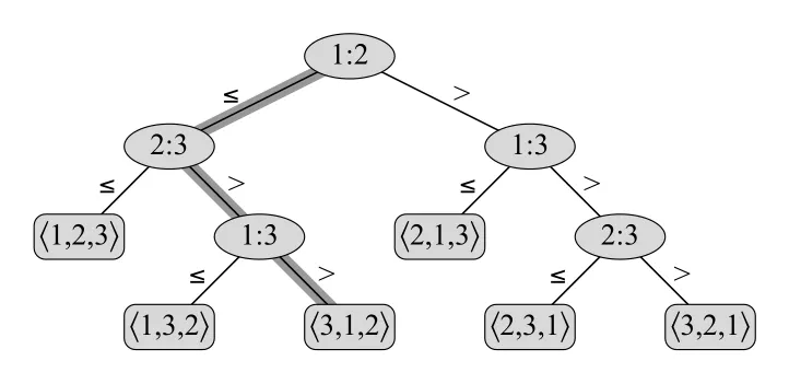Figure 8.1 · PDF p. 213 · 세 원소 insertion sort의 decision tree와 가능한 $3!$ permutations

Figure 8.1에서 internal node $i:j$ 는 $a_{i} \le a_{j}$ 비교를 뜻한다. 어떤 input에 대해 sorting algorithm을 실행하면 root에서 시작해 comparison 결과에 따라 leaf까지 내려간다. Leaf에는 예를 들어 $\langle 3,1,2\rangle$ 처럼 sorted order가 permutation으로 표시된다.

정확한 comparison sort라면 가능한 모든 input order를 올바르게 처리해야 하므로, $n$ 개 distinct elements의 가능한 모든 permutations가 reachable leaf로 나타나야 한다. 가능한 permutation 수는

n!

개다.

Worst-case lower bound

Decision tree에서 root에서 어떤 reachable leaf까지의 path length는 해당 input에서 수행한 comparison 수다. 따라서 tree height는 worst-case comparison 수다.

Height가 $h$ 인 binary tree는 leaf를 최대

2^{h}

개 가질 수 있다. Correct comparison sort의 decision tree에는 최소 $n!$ 개의 reachable leaves가 필요하므로

n! \le 2^{h}

이고, 양변에 log를 취하면

h \ge \lg(n!)

이다. Stirling approximation 또는 CLRS의 식 (3.19)에 의해

\lg(n!) = \Omega(n \lg n)

이므로 다음 theorem이 나온다.

\begin{aligned} Any comparison sort algorithm requires \Omega(n \lg n) \\ \text{comparisons in the worst case.} \end{aligned}

의미

이 lower bound는 comparison sort model 안에서는 merge sort와 heapsort가 asymptotically optimal하다는 뜻이다. 이미 $O(n \lg n)$ upper bound를 달성하므로, comparison만 사용하는 알고리즘으로는 asymptotic하게 더 빠른 worst-case sorting을 만들 수 없다.

하지만 이 결론은 comparison sort에만 해당한다. Counting sort, radix sort, bucket sort는 key range, digit structure, input distribution 같은 추가 구조를 사용해 comparison lower bound를 우회한다.

8.2 Counting sort

가정과 기본 아이디어

counting sort는 n개의 input elements가 모두 integer이고, 각 값이 범위

0..k

안에 있다고 가정한다. 특히 $k = O(n)$ 이면 전체 running time이 $\Theta(n)$ 이 된다.

Counting sort의 핵심 아이디어는 비교하지 않고 “각 값보다 작거나 같은 원소가 몇 개 있는지”를 세어 output position을 직접 계산하는 것이다. 예를 들어 17개의 elements가 x보다 작다면, distinct elements 상황에서 x는 output position 18에 놓인다. Equal values가 있으면 같은 position에 몰리지 않도록 count를 하나씩 줄여가며 배치한다.

사용하는 arrays:

$A[1..n]$ : input array
$B[1..n]$ : sorted output array
$C[0..k]$ : count와 prefix sum을 저장하는 temporary array

COUNTING-SORT procedure

COUNTING-SORT(A, B, k)
1  let C[0..k] be a new array
2  for i = 0 to k
3      C[i] = 0
4  for j = 1 to A.length
5      C[A[j]] = C[A[j]] + 1
6  // C[i] now contains the number of elements equal to i.
7  for i = 1 to k
8      C[i] = C[i] + C[i-1]
9  // C[i] now contains the number of elements less than or equal to i.
10 for j = A.length downto 1
11     B[C[A[j]]] = A[j]
12     C[A[j]] = C[A[j]] - 1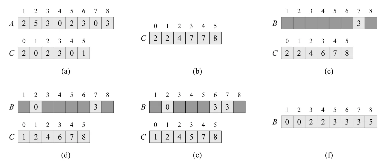

Figure 8.2 · PDF p. 216 · COUNTING-SORT에서 count array C가 frequency에서 prefix sum으로 바뀌고 output B를 채우는 과정

Figure 8.2는 세 단계를 보여준다.

$C[i]$ 가 value $i$ 의 frequency를 저장한다.
누적합 후 $C[i]$ 가 $\le i$ 인 elements 수를 저장한다.
Input을 뒤에서 앞으로 보며 B[C[A[j]]]에 배치하고 C[A[j]]를 감소시킨다.

C array의 의미 변화

Counting sort에서 C는 중간에 의미가 바뀐다.

시점	$C[i]$ 의 의미
line 5 이후	input에서 값이 정확히 $i$ 인 elements 수
line 8 이후	input에서 값이 $i$ 이하인 elements 수
line 10-12 중	값 $i$ 가 다음에 들어갈 output position 바로 앞/현재 경계

Line 8 이후 $C[i]$ 가 “ $i$ 이하 elements 수”가 되기 때문에, 값 $i$ 의 마지막 occurrence가 들어갈 수 있는 output position을 바로 알 수 있다. 예를 들어 $C[3] = 7$ 이면 값 $3$ 이하인 원소가 7개 있으므로, 값 $3$ 의 어떤 occurrence는 position 7 이하에 들어가야 한다.

Stability가 왜 생기는가

Counting sort는 stable sort다. 즉 같은 key를 가진 elements가 input에서 나온 상대 순서를 output에서도 유지한다. 이 성질은 line 10에서 input을

j = A.length downto 1

로 뒤에서 앞으로 순회하기 때문에 생긴다.

같은 value $v$ 를 가진 두 elements가 input에서 $A[a]$ , $A[b]$ 이고 $a < b$ 라고 하자. 뒤에서 앞으로 보므로 $A[b]$ 가 먼저 output의 더 뒤쪽 위치에 놓이고, $C[v]$ 가 감소한다. 이후 $A[a]$ 가 그보다 앞 위치에 놓인다. 결과적으로 input에서 먼저 나온 $A[a]$ 가 output에서도 먼저 나온다.

Stability는 satellite data가 붙은 records를 정렬할 때 중요하다. 예를 들어 key만 같고 나머지 정보가 다른 records의 상대 순서가 보존되어야 할 수 있다. Chapter 8에서는 특히 radix sort의 correctness를 위해 counting sort의 stability가 필수다.

시간복잡도와 lower bound 우회

각 loop의 비용은 다음과 같다.

\begin{aligned} \text{initialize C:} \Theta(k) \\ \text{count frequencies:} \Theta(n) \\ \text{prefix sums:} \Theta(k) \\ \text{write output:} \Theta(n) \end{aligned}

따라서 total running time은

\Theta(n + k)

이고, $k = O(n)$ 이면

\Theta(n)

이다.

Counting sort가 $\Omega(n \lg n)$ lower bound를 깨는 이유는 comparison sort가 아니기 때문이다. Input elements끼리 비교하지 않고, element value를 array index로 사용한다. 이 때문에 key range 0..k가 너무 크면 memory와 time이 커지고, k가 작거나 $O(n)$ 일 때 빛난다.

8.3 Radix sort

LSD부터 정렬하는 역직관

radix sort는 여러 digit으로 이루어진 keys를 digit별로 정렬한다. 원문은 card-sorting machines를 예로 든다. 기계는 한 번에 한 column만 볼 수 있으므로, d-digit number를 정렬하려면 digit별 sorting을 반복해야 한다.

처음 생각하기 쉬운 방식은 most significant digit부터 정렬하고, 각 bin을 recursive하게 다시 정렬하는 것이다. 하지만 이는 intermediate piles가 많아 관리가 복잡하다. Radix sort는 반대로 least significant digit, 즉 가장 덜 중요한 digit부터 정렬한다.

순서:

가장 낮은 자리 digit으로 stable sort
두 번째 낮은 자리 digit으로 stable sort
…
가장 높은 자리 digit까지 반복

이 과정을 마치면 전체 d-digit keys가 정렬된다.

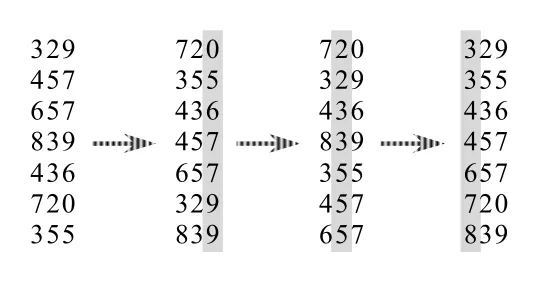Figure 8.3 · PDF p. 219 · 3자리 숫자들을 least significant digit부터 stable sort하는 radix sort 과정

Figure 8.3에서는 3-digit numbers가 일의 자리, 십의 자리, 백의 자리 순으로 정렬된다. 각 pass는 해당 digit만 기준으로 정렬하지만, 이전 pass에서 만들어 둔 lower-order digit의 ordering은 stable sort 덕분에 보존된다.

왜 stability가 필수인가

Radix sort의 correctness는 intermediate sort가 stable이라는 사실에 의존한다. 예를 들어 day, month, year로 구성된 dates를 정렬한다고 하자. Stable sort를 사용해

day \to month \to year

순서로 정렬하면, 마지막 year sort에서 같은 year를 가진 records 안에서는 이전 month ordering이 유지되고, 같은 month 안에서는 이전 day ordering이 유지된다.

즉 i번째 digit까지 정렬한 뒤에는 lower i digits 기준으로 이미 정렬되어 있다는 invariant가 유지된다. 다음 digit을 stable sort하면 새 digit 기준으로 묶이되, 같은 digit 값 내부에서는 이전 lower digits ordering이 보존된다.

RADIX-SORT procedure

원문은 digit 1을 lowest-order digit, digit d를 highest-order digit으로 둔다.

RADIX-SORT(A, d)
1  for i = 1 to d
2      use a stable sort to sort array A on digit i

여기서 stable sort로 counting sort를 쓰는 것이 자연스럽다. 각 digit이 $0..k-1$ 범위라면 한 pass의 비용은 $\Theta(n+k)$ 다.

Lemma 8.3:

\begin{aligned} n개의 d-digit numbers, \\ \text{각 digit이 최대 k개 값 중 하나,} \\ stable sort가 \Theta(n+k)이면 \\ RADIX-SORT &= \Theta(d(n+k)) \end{aligned}

특히 d가 constant이고 $k = O(n)$ 이면 radix sort는 linear time이다.

b-bit keys와 r-bit digits

컴퓨터에서는 key를 bit 단위로 잘라 digit으로 볼 수 있다. n개의 b-bit numbers를 정렬하고, 한 digit을 r bits로 잡는다고 하자.

digit 수: $d = \lceil b/r \rceil$
각 digit의 가능한 값 수: $2^{r}$
counting sort 한 pass 비용: $\Theta(n + 2^{r})$

따라서 running time은

\Theta((b/r)(n + 2^{r}))

이다.

$r$ 은 trade-off다.

$r$ 선택	효과
작게 잡음	digit 수 $b/r$ 가 많아져 pass 수 증가
크게 잡음	$2^{r}$ 크기의 count array가 커지고 pass당 비용 증가
$r \approx \lg n$	$2^{r} \approx n$ 이라 counting sort pass가 $\Theta(n)$ 이고 pass 수가 $b/\lg n$

원문은 다음처럼 정리한다.

$b < \lfloor \lg n \rfloor$ 이면 $r = b$ 를 선택해 한 pass로 $\Theta(n)$ 에 정렬할 수 있다.
$b \ge \lfloor \lg n \rfloor$ 이면 $r = \lfloor \lg n \rfloor$ 이 constant factor 안에서 좋은 선택이며, running time은 $\Theta(bn / \lg n)$ 이다.

Radix sort vs quicksort

겉으로 보면 $b = O(\lg n)$ 이고 $r \approx \lg n$ 이면 radix sort는 $\Theta(n)$ 으로, quicksort의 expected $\Theta(n \lg n)$ 보다 좋아 보인다. 하지만 실제 선택은 더 복잡하다.

Radix sort의 각 pass는 counting array 초기화와 memory access가 필요하다.
Counting sort 기반 radix sort는 in-place가 아니다.
Quicksort는 hardware caches를 더 잘 활용하는 경우가 많다.
Key representation, machine architecture, memory pressure, implementation constant가 실제 성능을 좌우한다.

따라서 radix sort는 theoretical linear time이 가능하지만, 항상 comparison sort보다 practical하게 우월하다고 말할 수는 없다.

8.4 Bucket sort

입력 가정: uniform distribution

Bucket sort는 counting sort처럼 input에 대한 강한 가정을 이용해 comparison lower bound를 피한다. Counting sort가 “key가 작은 integer range 0..k에 있다”는 가정을 쓰는 반면, bucket sort는 input이 random process에 의해 생성되며 interval [0, 1) 위에 uniformly and independently distributed되어 있다고 가정한다.

이 가정의 의미는 다음과 같다.

각 원소 $A[i]$ 는 $0 \le A[i] < 1$ 이다.
[0,1)을 같은 크기의 n개 subinterval로 나누면, 각 원소가 어느 bucket에 들어갈 확률은 거의 같다.
원소들이 independent하므로 한 bucket에 원소가 몰릴 가능성은 평균적으로 작다.

따라서 전체 정렬을 한 번에 comparison sort로 처리하지 않고, 값을 bucket에 흩뿌린 뒤 각 bucket 내부만 정렬한다.

Bucket sort의 구조

n개의 bucket을 만들고, interval [0,1)을 다음처럼 나눈다.

\begin{aligned} \text{B[0] :} [0/n, 1/n) \\ \text{B[1] :} [1/n, 2/n) \\ \text{...} \\ \text{B[i] :} [i/n, (i+1)/n) \\ \text{...} \\ \text{B[n-1] :} [(n-1)/n, 1) \end{aligned}

원소 $A[i]$ 는

\lfloor n A[i] \rfloor

번째 bucket으로 들어간다. 이후 각 bucket의 linked list를 insertion sort로 정렬하고, bucket index 순서대로 concatenate하면 전체 sorted output이 된다.

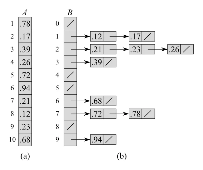Figure 8.4 · PDF p. 222 · [0,1) 입력 10개를 10개 bucket에 분산하고 bucket 순서대로 연결하는 BUCKET-SORT

Figure 8.4에서 $n = 10$ 이므로 $B[0]$ 은 [0, .1), $B[1]$ 은 [.1, .2), …, $B[9]$ 는 [.9, 1) 범위를 담당한다. 예를 들어 .78은 $\lfloor 10 \cdot .78 \rfloor = 7$ 이므로 $B[7]$ 로 들어간다.

BUCKET-SORT procedure

BUCKET-SORT(A)
1  n = A.length
2  let B[0..n-1] be a new array
3  for i = 0 to n-1
4      make B[i] an empty list
5  for i = 1 to n
6      insert A[i] into list B[floor(n A[i])]
7  for i = 0 to n-1
8      sort list B[i] with insertion sort
9  concatenate the lists B[0], B[1], ..., B[n-1] together in order

Auxiliary array $B[0..n-1]$ 의 각 entry는 bucket을 나타내는 linked list다. CLRS가 linked list를 쓰는 이유는 각 bucket에 몇 개의 원소가 들어갈지 미리 모르기 때문이다.

Correctness

Bucket sort의 correctness는 bucket index가 값의 범위 순서를 보존한다는 점에 있다.

두 원소 $A[i] \le A[j]$ 를 생각하자. 그러면

\lfloor n A[i] \rfloor \le \lfloor n A[j] \rfloor

이다. 가능한 경우는 두 가지다.

경우	처리 방식
두 원소가 같은 bucket에 들어감	line 7-8의 insertion sort가 bucket 내부 순서를 맞춘다
두 원소가 다른 bucket에 들어감	더 작은 값은 더 낮은 bucket index에 있고, line 9의 concatenate 순서가 전체 순서를 맞춘다

즉 bucket 내부 정렬과 bucket 간 index 순서가 합쳐져 전체 sorted order가 된다.

Average-case running time 분석

Line 8의 insertion sort를 제외한 모든 작업은 worst case에서도 $O(n)$ 이다. 핵심은 bucket 내부 정렬 비용의 합이다.

$n_{i}$ 를 bucket $B[i]$ 에 들어간 원소 수라고 하자. Insertion sort는 bucket 크기에 대해 quadratic time이므로 전체 running time은

T(n) = \Theta(n) + \sum_{i=0}^{n-1} O(n_{i}^{2})

이다. 이제 expectation을 취하면 linearity of expectation에 의해

E[T(n)] = \Theta(n) + \sum_{i=0}^{n-1} O(E[n_{i}^{2}])

만 보이면 된다. Uniform independent input에서는 각 bucket에 대해

E[n_{i}^{2}] = 2 - 1/n < 2

가 성립한다.

이 계산은 indicator random variables로 보인다. $X_{ij}$ 를 “ $A[j]$ 가 bucket i에 들어가면 1, 아니면 0”인 indicator라고 하면

n_{i} = \sum_{j=1}^{n} X_{ij}

이고, 각 원소가 특정 bucket에 들어갈 확률은 $1/n$ 이다. 따라서

E[X_{ij}^{2}] = 1/n

이다. $j \ne k$ 일 때 두 원소의 bucket 배정은 independent이므로

E[X_{ij} X_{ik}] = E[X_{ij}] E[X_{ik}] = 1/n^{2}

이다. 이를 제곱 전개에 대입하면

\begin{aligned} E[n_{i}^{2}] \\ = \sum_{j} E[X_{ij}^{2}] + \sum_{j} \sum_{k != j} E[X_{ij} X_{ik}] \\ = n(1/n) + n(n-1)(1/n^{2}) \\ = 1 + (n-1)/n \\ = 2 - 1/n \end{aligned}

이다. 결국

E[T(n)] = \Theta(n) + n \cdot O(2 - 1/n) = \Theta(n)

이므로 bucket sort의 average-case running time은 $\Theta(n)$ 이다.

Worst case와 가정의 의미

Bucket sort가 항상 linear time인 것은 아니다. 모든 원소가 한 bucket에 몰리면 line 8에서 insertion sort가 n개 원소를 한 번에 정렬하므로 worst-case running time은

\Theta(n^{2})

이다.

따라서 bucket sort의 성능 보장은 “input이 uniform distribution에서 independent하게 나온다”는 모델에 기대고 있다. 다만 원문은 uniform distribution이 아니더라도

\sum_{i} n_{i}^{2} = O(n)

이 유지되는 input distribution이라면 equation (8.1)에 의해 linear average-case time이 가능하다고 설명한다. 핵심은 bucket마다 작은 list가 생기는 것이지, 꼭 완벽한 uniformity 자체가 목적은 아니다.

Bucket sort의 단순 worst-case 개선

Exercise 8.4-2가 암시하듯, bucket 내부 정렬을 insertion sort 대신 $O(m \lg m)$ comparison sort로 바꾸면 worst case를 개선할 수 있다. 모든 원소가 한 bucket에 몰려도 그 bucket을 $O(n \lg n)$ 에 정렬하므로 전체 worst-case는 $O(n \lg n)$ 이 된다. Average case에서는 bucket 크기가 작게 유지되므로 linear average-case의 장점도 보존할 수 있다.

Uniform하지 않은 분포로의 확장

Exercise 8.4-4와 8.4-5는 bucket sort를 “균등한 bucket 폭”으로만 이해하면 부족하다는 점을 보여 준다.

Unit circle 안의 points를 origin으로부터의 distance $d_{i} = \sqrt{x_{i}^{2} + y_{i}^{2}}$ 기준으로 정렬할 때, 점은 면적에 비례해 uniform하다. 반지름 r 이하의 면적은 $\pi r^{2}$ 에 비례하므로 distance 자체가 균등하지 않다. Bucket 경계는 distance가 아니라 area가 균등해지도록 잡아야 한다.
Continuous probability distribution function $P(x) = \Pr\left\{X \le x\right\}$ 를 $O(1)$ 에 계산할 수 있다면, 값 x를 $P(x)$ 로 변환해 [0,1)의 uniform variable처럼 다룰 수 있다. 이 idea는 cumulative distribution function, 즉 CDF를 이용한 bucketization이다.

즉 bucket sort의 본질은 “원소가 각 bucket에 균형 있게 들어가도록 bucket index function을 설계하는 것”이다.

Problems and chapter notes

Problems의 확장 포인트

Chapter 8의 Problems는 본문 알고리즘을 단순 응용하기보다, sorting lower bound와 model assumption을 더 넓게 밀어붙인다.

문제	핵심 주제	본문과의 연결
8-1 Probabilistic lower bounds on comparison sorting	deterministic/randomized comparison sort의 average lower bound	decision-tree model, $\Omega(n \lg n)$
8-2 Sorting in place in linear time	$O(n)$ , stable, in-place 세 조건의 충돌	counting sort, radix sort의 stability/space trade-off
8-3 Sorting variable-length items	총 digit/character 수가 `n`일 때 linear sorting	radix sort 사고방식
8-4 Water jugs	직접 비교 가능한 쌍이 제한된 matching 문제	comparison lower bound, randomized partitioning
8-5 Average sorting	`k-sorted`라는 약한 정렬 조건	sorting lower bound의 변형
8-6 Lower bound on merging sorted lists	merging에 필요한 comparison lower bound	merge sort의 merge subroutine
8-7 The 0-1 sorting lemma and columnsort	oblivious compare-exchange algorithm 증명법	sorting networks, columnsort

Figure 8.5는 Problem 8-7의 columnsort 절차를 보여 주는 그림이다. Chapter 8 본문 핵심 알고리즘인 counting sort, radix sort, bucket sort의 이해에는 직접 필요하지 않으므로 이미지로 포함하지 않았다. 다만 0-1 sorting lemma, oblivious compare-exchange algorithm, columnsort, column-major order는 검색 가능한 용어로 남겨 둔다.

Chapter notes에서 남길 점

Chapter notes는 다음 역사적, 이론적 연결을 알려 준다.

decision-tree model은 comparison sort lower bound를 설명하는 표준 모델이다.
counting sort와 counting sort를 radix sort에 결합하는 idea는 오래된 punch-card/card-sorting 맥락과 연결된다.
bucket sort의 기본 idea도 오래된 distribution-based sorting 기법이다.
b-bit integers를 $o(n \lg n)$ 에 sorting하는 연구는 fusion tree, word-RAM model, multiplication, hashing, exponential search trees 등 computation model에 민감하다.
이런 integer sorting algorithms는 이론적으로 중요하지만, 구현 복잡도와 constant factor 때문에 실무 sorting algorithm을 바로 대체한다고 보기는 어렵다.

복잡도

알고리즘/결과	시간 복잡도	공간/조건	핵심 이유
Comparison sort lower bound	worst case $\Omega(n \lg n)$	comparison model	decision tree에 $n!$ reachable leaves 필요
Counting sort	$\Theta(n+k)$	$A[1..n]$ , $B[1..n]$ , $C[0..k]$	key range를 count array index로 사용
Counting sort, $k = O(n)$	$\Theta(n)$	integer keys in `0..k`	comparison으로 order를 찾지 않음
Radix sort	$\Theta(d(n+k))$	`d` digits, digit range $0..k-1$ , stable sort 필요	낮은 자리부터 digit별 stable sorting
Radix sort on $b$ -bit keys	$\Theta((b/r)(n + 2^{r}))$	digit size $r$ bits	pass 수와 counting array 크기의 trade-off
Bucket sort average case	$\Theta(n)$	independent uniform `[0,1)` 또는 $\sum_{i} n_{i}^{2} = O(n)$	bucket 내부 expected square size가 constant
Bucket sort worst case	$\Theta(n^{2})$	insertion sort 사용 시	모든 원소가 한 bucket에 몰릴 수 있음

연결 관계

Chapter 2의 insertion sort는 bucket sort에서 작은 bucket 내부를 정렬하는 subroutine으로 다시 등장한다.
Chapter 5의 indicator random variables와 linearity of expectation은 bucket sort average-case analysis의 핵심 도구다.
Chapter 6의 heapsort, Chapter 7의 quicksort는 comparison sort 범주에 있으므로 $\Omega(n \lg n)$ lower bound의 적용을 받는다.
Counting sort의 stability는 radix sort correctness의 전제다.
Chapter 10의 linked list는 bucket array $B[0..n-1]$ 의 각 bucket을 구현하는 자료구조로 연결된다.
Appendix C의 uniform distribution, expectation, indicator random variables가 bucket sort 분석에 직접 쓰인다.

오해하기 쉬운 내용

$\Omega(n \lg n)$ lower bound는 모든 sorting algorithm에 대한 말이 아니라 comparison sort에 대한 말이다.
Counting sort가 linear time인 이유는 비교를 잘해서가 아니라 key 값을 array index로 사용하기 때문이다.
Counting sort는 stable하지만 일반적인 형태에서는 in-place가 아니다.
Radix sort는 lower digit부터 정렬한다. 이때 중간 정렬이 stable하지 않으면 lower digit ordering이 깨진다.
Radix sort의 $\Theta(n)$ 가능성은 digit 수 d와 digit range k가 작거나 적절히 제한될 때의 이야기다.
Bucket sort의 $\Theta(n)$ 은 average-case 결과다. Worst case는 원소가 한 bucket에 몰리면 $\Theta(n^{2})$ 이다.
Bucket sort에서 bucket 폭을 항상 같게 잡아야 하는 것은 아니다. Input distribution에 맞춰 bucket index function을 설계하는 것이 핵심이다.
stable, in-place, linear time은 동시에 쉽게 만족되지 않는다. Problem 8-2는 이 trade-off를 직접 묻는다.

면접 질문

Comparison sort의 decision-tree model에서 왜 reachable leaf가 최소 $n!$ 개 필요할까?
$n! \le 2^{h}$ 에서 어떻게 $\Omega(n \lg n)$ lower bound가 나오는가?
Counting sort가 comparison sort lower bound를 피하는 이유는 무엇인가?
COUNTING-SORT에서 array C는 line 7 이후 어떤 의미를 가지는가?
Counting sort가 stable하려면 왜 input을 뒤에서 앞으로 순회해야 하는가?
Radix sort에서 intermediate sort가 stable하지 않으면 어떤 문제가 생기는가?
b-bit integer를 r-bit digit으로 나누면 radix sort의 시간은 왜 $\Theta((b/r)(n + 2^{r}))$ 인가?
Bucket sort의 expected time 분석에서 왜 $E[n_{i}^{2}]$ 를 계산해야 하는가?
Bucket sort의 average-case $\Theta(n)$ 과 worst-case $\Theta(n^{2})$ 는 어떤 input distribution 차이에서 발생하는가?
stable, in-place, linear time 조건이 sorting algorithm 설계에서 어떤 trade-off를 만드는가?