Chapter 14. Augmenting Data Structures

개요

Chapter 14는 textbook data structure를 완전히 새로 만들기보다, 기존 구조에 추가 정보를 저장해 필요한 operation을 빠르게 만드는 augmenting data structures 기법을 다룬다. 핵심은 “추가 field를 넣는 것” 자체가 아니라, 기존 INSERT, DELETE, ROTATE 같은 ordinary operations가 그 추가 정보를 효율적으로 유지할 수 있느냐이다.

이 장의 두 대표 예시는 모두 Chapter 13의 red-black trees를 기반으로 한다.

order-statistic tree: 각 node에 subtree size x.size를 저장해 i번째 smallest element와 rank를 $O(\lg n)$ 에 찾는다.
interval tree: 각 node에 interval과 subtree maximum high endpoint x.max를 저장해 query interval과 겹치는 interval을 $O(\lg n)$ 에 찾는다.

Chapter 14의 큰 메시지는 “균형 search tree + 유지 가능한 보조 정보”가 다양한 고급 dynamic-set operation을 만드는 표준 설계 패턴이라는 것이다.

핵심 개념

용어	의미	검색 키워드
augmentation	기존 data structure에 추가 정보를 저장해 operation을 확장하는 기법	augmenting data structures
order statistic	set에서 `i`번째로 작은 원소	order statistic
order-statistic tree	`x.size`를 저장하는 augmented red-black tree	order-statistic tree
subtree size	node `x`를 root로 하는 subtree의 internal node 수	`x.size`, `T.nil.size`
rank	inorder walk에서 element가 출력되는 위치	rank, `OS-RANK`
select	rank `i`를 가진 element를 찾는 operation	`OS-SELECT`
rotation maintenance	rotation 후 추가 attribute를 local하게 갱신하는 작업	`LEFT-ROTATE`, `RIGHT-ROTATE`
augmentation theorem	red-black tree에 local field를 추가해도 asymptotic update time을 유지한다는 정리	Theorem 14.1
interval tree	intervals를 저장하고 overlap query를 지원하는 augmented red-black tree	interval tree
max endpoint	subtree 안 interval들의 high endpoint 최댓값	`x.max`

세부 정리

14.1 Dynamic order statistics

Order-statistic tree의 목적

Chapter 9에서 ith order statistic은 n개 원소 중 i번째로 작은 key를 뜻했다. Unordered set에서는 임의의 order statistic을 $O(n)$ time에 찾을 수 있었다. 하지만 dynamic set에서는 insertion/deletion이 계속 일어나므로, 매번 전체 set에서 다시 selection을 수행하면 비효율적이다.

order-statistic tree는 red-black tree를 augment하여 다음 operation을 모두 $O(\lg n)$ 에 지원한다.

OS-SELECT(T.root, i): 현재 set에서 i번째 smallest element를 찾는다.
OS-RANK(T, x): node x가 inorder order에서 몇 번째인지 찾는다.
ordinary red-black tree operations: SEARCH, INSERT, DELETE도 $O(\lg n)$ 유지.

`x.size` attribute

Order-statistic tree는 각 internal node x에 x.size를 추가한다.

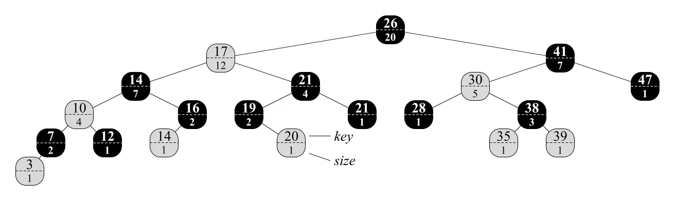\begin{aligned} x.size &= number of internal nodes in subtree rooted at x \\ T.nil.size &= 0 \\ x.size &= x.left.size + x.right.size + 1 \end{aligned}

Figure 14.1 · PDF p. 361 · 각 node에 subtree size를 저장한 order-statistic tree

Figure 14.1은 red-black tree의 각 node에 key와 size를 함께 표시한다. size는 sentinel을 제외한 internal nodes만 센다. 이 field 덕분에 특정 node의 left subtree에 몇 개의 원소가 있는지 즉시 알 수 있고, rank 기반 navigation이 가능해진다.

Order-statistic tree는 keys가 distinct하다고 요구하지 않는다. Duplicate keys가 있으면 “rank of key value”는 애매해질 수 있으므로, CLRS는 element의 rank를 inorder walk에서 출력되는 위치로 정의한다. 예를 들어 같은 key 14가 두 번 나오더라도, black node의 14와 red node의 14는 inorder position이 다르므로 각각 rank가 다르다.

OS-SELECT: rank로 node 찾기

OS-SELECT(x, i)는 subtree rooted at x에서 i번째 smallest key를 가진 node pointer를 반환한다. 전체 tree에서 찾으려면 OS-SELECT(T.root, i)를 호출한다.

OS-SELECT(x, i)
1  r = x.left.size + 1
2  if i == r
3      return x
4  elseif i < r
5      return OS-SELECT(x.left, i)
6  else return OS-SELECT(x.right, i - r)

Line 1의 $r = x.left.size + 1$ 은 subtree rooted at x 안에서 x 자신의 rank다. Left subtree에 있는 모든 node가 inorder order에서 x보다 먼저 나오고, 그 다음이 x이기 때문이다.

세 경우는 자연스럽다.

조건	의미	다음 행동
$i = r$	$x$ 가 찾는 rank	$x$ 반환
$i < r$	찾는 node가 left subtree에 있음	`OS-SELECT(x.left, i)`
$i > r$	찾는 node가 right subtree에 있음	`OS-SELECT(x.right, i-r)`

$i > r$ 일 때 $i-r$ 로 바꾸는 이유는 right subtree 안에서는 $x$ 와 left subtree의 $r$ 개 원소를 제외한 rank로 다시 계산해야 하기 때문이다.

Figure 14.1에서 17번째 smallest element를 찾는 예시는 다음처럼 진행된다.

\begin{aligned} x &= 26, i = 17, left.size = 12 \to r = 13 \to go right with i = 4 \\ x &= 41, i = 4, left.size = 5 \to r = 6 \to go left with i = 4 \\ x &= 30, i = 4, left.size = 1 \to r = 2 \to go right with i = 2 \\ x &= 38, i = 2, left.size = 1 \to r = 2 \to return 38 \end{aligned}

각 recursive call은 tree에서 한 level 내려가므로, red-black tree height bound에 의해 OS-SELECT는 $O(\lg n)$ time이다.

OS-RANK: node로 rank 찾기

OS-RANK(T, x)는 order-statistic tree T와 node pointer x를 받아, x가 inorder order에서 몇 번째인지 반환한다.

OS-RANK(T, x)
1  r = x.left.size + 1
2  y = x
3  while y != T.root
4      if y == y.p.right
5          r = r + y.p.left.size + 1
6      y = y.p
7  return r

초기값 $r = x.left.size + 1$ 은 subtree rooted at x 안에서 x의 rank다. 이후 y를 parent 방향으로 올리면서, x 앞에 추가로 놓이는 nodes가 있는지 계산한다.

핵심 invariant는 다음과 같다.

At the start of each loop iteration,
r is the rank of x within the subtree rooted at y.

y가 parent의 left child라면 parent와 parent의 right subtree는 inorder에서 x 뒤에 오므로 더할 것이 없다. y가 parent의 right child라면 parent의 left subtree 전체와 parent 자신이 x보다 앞에 온다. 그래서 line 5에서 y.p.left.size + 1을 더한다.

Figure 14.1에서 key 38 node의 rank를 구하면 loop top의 (y.key, r) 값이 다음처럼 변한다.

(38, 2) \to (30, 4) \to (41, 4) \to (26, 17)

따라서 rank는 17이다. OS-RANK는 parent pointer를 따라 한 level씩 올라가므로 $O(\lg n)$ time이다.

Maintaining subtree sizes

OS-SELECT와 OS-RANK가 빠른 이유는 x.size가 항상 정확하다는 가정 때문이다. 따라서 insertion/deletion/rotation 중 size를 효율적으로 유지해야 한다.

Red-black insertion의 첫 단계는 root에서 leaf position까지 내려가며 새 node를 붙인다. 이때 traversed path의 모든 node x에 대해 x.size를 1씩 증가시키면 된다. 새 node의 size는 1이다. Path length가 $O(\lg n)$ 이므로 추가 비용도 $O(\lg n)$ 이다.

Insertion fixup의 structural changes는 rotations뿐이고, red-black insertion은 최대 두 번 rotation한다. Rotation은 local operation이므로 size 갱신도 local하다.

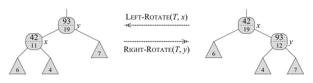Figure 14.2 · PDF p. 365 · rotation 후 영향을 받는 두 node의 subtree size 갱신

LEFT-ROTATE(T, x)에서 pivot node를 $y = x.right$ 라고 하면, rotation 후 y가 기존 x의 subtree root가 된다. 따라서 CLRS는 LEFT-ROTATE 끝에 다음 두 줄을 추가한다.

\begin{aligned} y.size &= x.size \\ x.size &= x.left.size + x.right.size + 1 \end{aligned}

$y.size = x.size$ 가 먼저인 이유는 rotation 전 x가 대표하던 subtree 전체를 rotation 후 y가 대표하기 때문이다. 그 다음 x의 children이 바뀐 상태에서 x.size를 다시 계산한다. RIGHT-ROTATE는 대칭적이다.

Deletion도 두 단계로 본다. 첫 단계에서 실제로 제거되거나 이동되는 node $y$ 의 original position부터 root까지 올라가며 size를 1씩 감소시킨다. 이 path도 $O(\lg n)$ 이다. 두 번째 fixup 단계의 rotations는 최대 세 번이고, 각 rotation의 size 갱신은 $O(1)$ 이다. 따라서 order-statistic tree의 insertion/deletion은 size 유지까지 포함해도 $O(\lg n)$ time이다.

14.1 Exercises에서 남길 포인트

OS-SELECT는 recursion 없이도 구현할 수 있다. 현재 node x와 rank i를 유지하면서, $r = x.left.size + 1$ 을 반복 계산해 left/right로 이동하면 된다. 이 iterative version도 path 하나만 내려가므로 $O(\lg n)$ 이다.

Distinct keys를 가정하면 OS-KEY-RANK(T, k)는 search와 rank 계산을 섞어 구현할 수 있다. Search 중 right로 내려갈 때마다 현재 node와 left subtree가 모두 k보다 작으므로 그 수를 누적한다. 이 아이디어는 OS-RANK가 parent 방향으로 올라가며 더하는 값을, root에서 내려가며 미리 더하는 방식이다.

ith successor of x는 OS-RANK(T, x)로 x의 rank r을 구한 뒤 OS-SELECT(T.root, r+i)를 호출하면 된다. 두 operation이 각각 $O(\lg n)$ 이므로 전체도 $O(\lg n)$ 이다.

14.2 How to augment a data structure

Augmentation의 4단계

Data structure augmentation은 algorithm design에서 자주 등장하는 패턴이다. 기존 구조를 그대로 쓰되, 추가 정보를 저장하고 그 정보를 유지해 새로운 operation을 빠르게 만든다. CLRS는 augmentation을 다음 네 단계로 정리한다.

단계	질문	order-statistic tree에서의 답
1. Choose an underlying data structure	어떤 기본 구조를 쓸 것인가?	red-black tree
2. Determine additional information	어떤 정보를 추가로 저장할 것인가?	subtree size `x.size`
3. Verify maintainability	기본 update 중 정보를 효율적으로 유지할 수 있는가?	path update + local rotation update
4. Develop new operations	추가 정보로 어떤 operation을 만들 것인가?	`OS-SELECT`, `OS-RANK`

이 단계는 기계적으로 순서대로만 진행하는 처방이 아니다. 실제 설계에서는 trial and error가 필요하다. 예를 들어 “각 node에 전체 tree에서의 rank를 저장하자”는 아이디어는 OS-SELECT, OS-RANK를 빠르게 만들 수 있어 보이지만, 새 minimum이 삽입되면 거의 모든 node의 rank가 바뀌어 유지 비용이 커진다. 반면 subtree size x.size는 insertion path와 rotation 주변에서만 바뀌므로 효율적으로 유지된다.

핵심 판단 기준은 다음과 같다.

additional information이 query를 빠르게 만드는가?
그리고 ordinary update가 그 정보를 싸게 유지할 수 있는가?

Theorem 14.1: Augmenting a red-black tree

Theorem 14.1은 red-black tree augmentation에서 step 3을 쉽게 확인하게 해주는 정리다.

Node x의 추가 attribute f가 x, x.left, x.right의 정보만으로 계산 가능하고, 필요하면 x.left.f, x.right.f에 의존해도 된다면, insertion/deletion 중 모든 node의 f 값을 유지해도 red-black tree의 $O(\lg n)$ update time을 asymptotically 악화시키지 않는다.

이를 수식처럼 쓰면 다음 형태다.

\begin{aligned} x.f &= g(x's own attributes, x.left's attributes, x.right's attributes) \\ \text{possibly using x.left.f and x.right.f} \end{aligned}

Order-statistic tree의 x.size가 정확히 이 조건을 만족한다.

x.size = x.left.size + x.right.size + 1

Theorem 14.1의 proof idea

증명의 핵심은 dependency가 아래에서 위로만 전파된다는 점이다. 어떤 node x의 f가 바뀌면 직접 영향을 받는 것은 x.p.f뿐이다. 그 다음에는 x.p.p.f가 영향을 받을 수 있고, 이런 식으로 root까지 올라간다. Red-black tree의 height는 $O(\lg n)$ 이므로, 한 local change의 영향을 전파하는 비용은 $O(\lg n)$ 이다.

Insertion은 두 phase로 본다.

Phase 1: 새 node x를 leaf position에 삽입한다. 새 node의 children은 T.nil이므로 x.f를 $O(1)$ 에 계산할 수 있다. 이후 변화가 ancestors로 전파되어 $O(\lg n)$ 이다.
Phase 2: red-black fixup에서 structural change는 rotations뿐이다. Insertion rotation 수는 최대 2번이고, 각 rotation 후 필요한 f propagation을 해도 총 $O(\lg n)$ 이다.

Deletion도 비슷하다.

Phase 1: node removal 또는 successor movement가 tree를 local하게 바꾼다. 그 변화가 ancestors로 전파되어 $O(\lg n)$ 이다.
Phase 2: delete fixup의 rotations는 최대 3번이고, 각 rotation 후 f를 유지해도 total $O(\lg n)$ 이다.

Theorem proof는 rotation 후 attribute 갱신 비용을 보수적으로 $O(\lg n)$ 으로 잡는다. 실제로 x.size처럼 많은 attributes는 rotation 주변 두 node만 다시 계산하면 되어 $O(1)$ 에 갱신된다. 따라서 theorem은 “이 정도 조건이면 적어도 asymptotic update time은 망치지 않는다”는 충분조건으로 이해하면 좋다.

Maintainable attribute와 그렇지 않은 attribute

Theorem 14.1의 조건은 “subtree-local”이다. x.f가 x와 children의 정보만으로 계산 가능해야 한다.

attribute idea	유지 가능성	이유
`x.size`	좋음	children sizes로 계산 가능
subtree max endpoint `x.max`	좋음	`x.int.high`, `x.left.max`, `x.right.max`로 계산 가능
black-height	가능	children의 black-height와 color에서 계산 가능
depth	나쁨	node의 ancestors에 의존하고 rotation 시 subtree 전체 depths가 바뀔 수 있음
global rank	나쁨	새 minimum 삽입 등으로 많은 nodes의 rank가 변함

이 distinction이 augmentation 설계의 감각이다. Query에 필요한 정보를 무작정 node에 저장하는 것이 아니라, update locality가 유지되는 형태로 재표현해야 한다.

14.2 Exercises에서 남길 포인트

MINIMUM, MAXIMUM, SUCCESSOR, PREDECESSOR를 $O(1)$ worst-case로 만들고 싶다면 node나 tree에 추가 pointers를 둘 수 있다. 예를 들어 tree-level pointer로 minimum/maximum을 유지하고, 각 node에 predecessor/successor pointer를 유지하면 query는 빨라진다. 다만 insertion/deletion 때 이 pointers를 정확히 갱신해야 하며, update asymptotic time을 악화시키지 않아야 한다.

RB-ENUMERATE(x, a, b)처럼 range 안의 keys를 모두 출력하는 operation은 새 attribute 없이도 $\Theta(m + \lg n)$ 에 가능하다. 먼저 lower bound $a$ 근처까지 search하고, 이후 successor 방향으로 $b$ 이하의 $m$ 개 keys를 출력하면 된다. 출력 자체가 $m$ 개이므로 $m$ 항은 피할 수 없다.

14.3 Interval trees

Interval과 overlap

interval tree는 intervals의 dynamic set을 유지하면서, query interval과 겹치는 interval 하나를 빠르게 찾기 위한 augmented red-black tree다. CLRS는 closed interval을 기본으로 사용한다.

\begin{aligned} i &= [t1, t2], where t1 \le t2 \\ i.low &= t1 \\ i.high &= t2 \end{aligned}

두 intervals i, i'가 overlap한다는 것은 교집합이 비어 있지 않다는 뜻이다.

i overlaps i' \Longleftrightarrow i.low \le i'.high and i'.low \le i.high

Open interval이나 half-open interval도 개념적으로 확장할 수 있지만, endpoint 포함 여부에 따라 inequality가 달라진다.

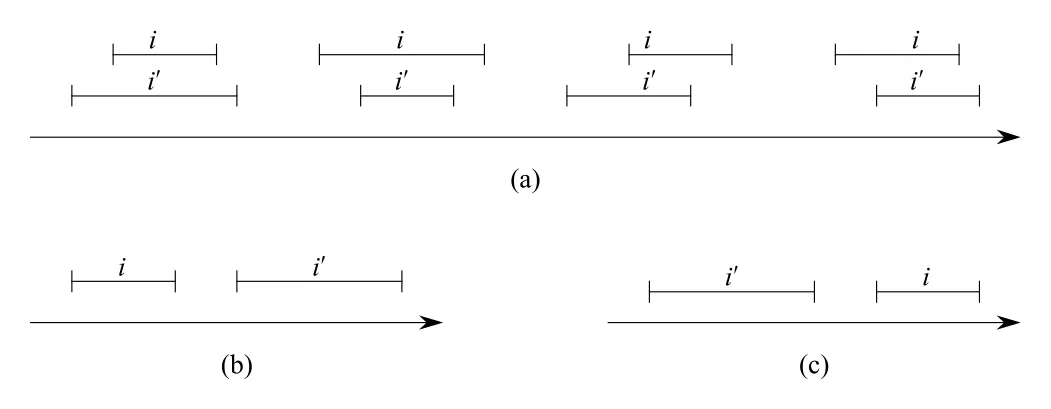Figure 14.3 · PDF p. 370 · 두 closed intervals의 overlap/non-overlap trichotomy

Figure 14.3의 interval trichotomy는 두 closed intervals i, i'에 대해 정확히 하나만 성립한다고 말한다.

경우	조건	의미
overlap	$i.low \le i'.high$ and $i'.low \le i.high$	두 intervals가 겹침
$i$ is left of $i'$	$i.high < i'.low$	$i$ 가 완전히 왼쪽
$i$ is right of $i'$	$i'.high < i.low$	$i$ 가 완전히 오른쪽

Interval tree의 구조

Interval tree는 각 node x에 interval x.int를 저장하고, x.int.low를 BST key로 사용한다. 따라서 inorder tree walk는 intervals를 low endpoint 기준 sorted order로 나열한다.

새 operation은 다음이다.

INTERVAL-INSERT(T, x): interval x.int를 가진 element x를 삽입한다.
INTERVAL-DELETE(T, x): element x를 제거한다.
INTERVAL-SEARCH(T, i): query interval i와 overlap하는 interval을 가진 node를 하나 반환한다. 없으면 T.nil을 반환한다.

Step 2의 additional information은 x.max다.

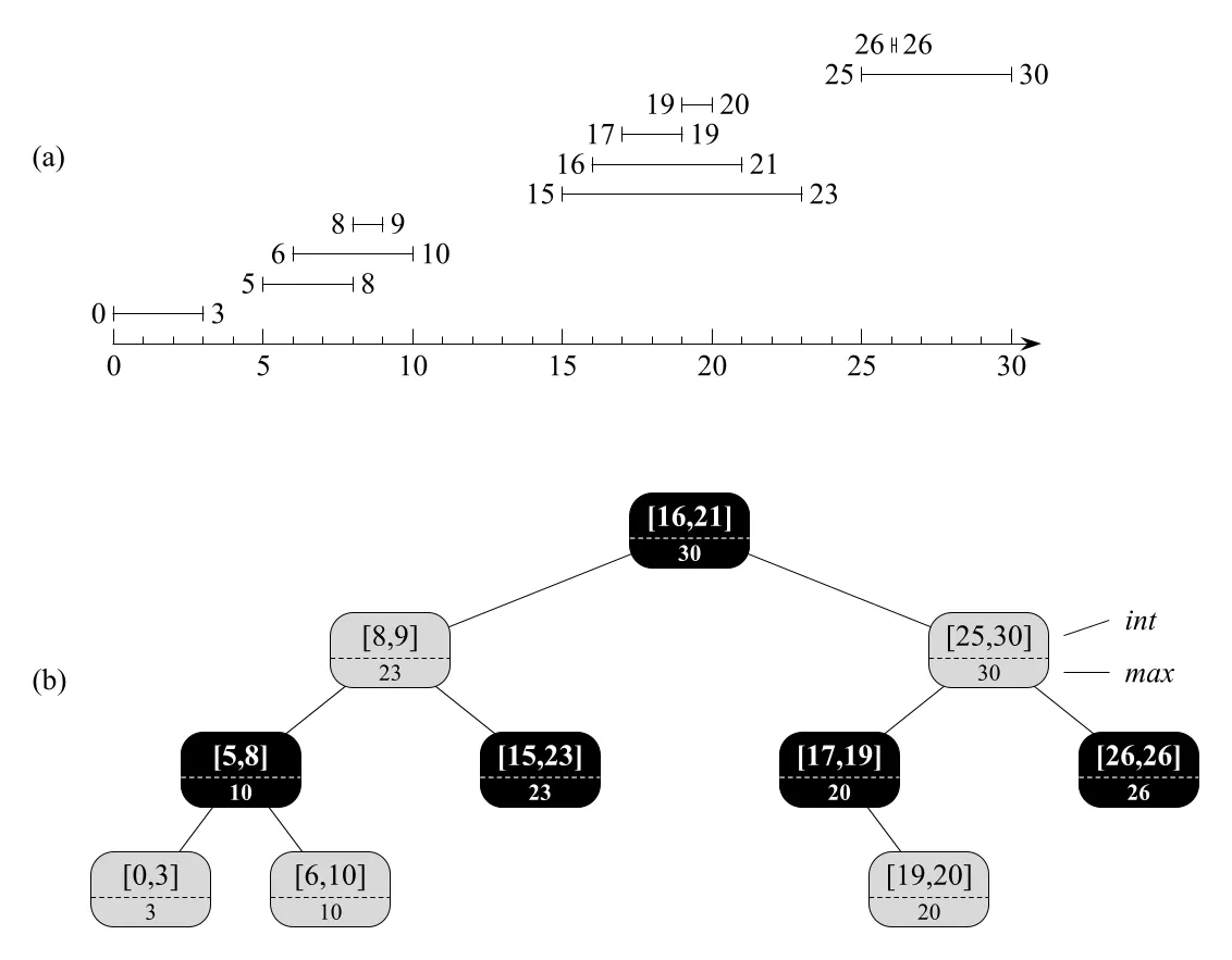\begin{aligned} x.\max &= maximum high endpoint among intervals in subtree rooted at x \\ x.\max &= \max(x.int.high, x.left.max, x.right.\max) \end{aligned}

Figure 14.4 · PDF p. 371 · interval을 low endpoint로 정렬하고 subtree max endpoint를 저장한 interval tree

Figure 14.4에서 각 node는 dashed line 위에 interval을, 아래에 subtree의 maximum high endpoint max를 표시한다. 예를 들어 어떤 node의 left subtree 안에 high endpoint가 큰 interval이 있다면, x.left.max가 그 가능성을 요약한다. Query는 이 값만 보고 left subtree에 overlap 후보가 있을 수 있는지 판단한다.

x.max는 x.int.high, x.left.max, x.right.max만으로 계산되므로 Theorem 14.1의 조건을 만족한다. 따라서 interval tree의 insertion/deletion은 x.max 유지까지 포함해도 $O(\lg n)$ 이다. 실제 rotation 후 max 갱신도 size와 비슷하게 영향받는 두 node를 local하게 다시 계산하면 되어 $O(1)$ 에 가능하다.

INTERVAL-SEARCH

INTERVAL-SEARCH(T, i)는 query interval i와 겹치는 interval을 가진 node 하나를 찾는다.

INTERVAL-SEARCH(T, i)
1  x = T.root
2  while x != T.nil and i does not overlap x.int
3      if x.left != T.nil and x.left.max >= i.low
4          x = x.left
5      else x = x.right
6  return x

Search는 root에서 시작해 한 path만 내려간다. 현재 node x의 interval이 i와 overlap하면 즉시 반환한다. 겹치지 않으면 left subtree에 overlap 후보가 있을 수 있는지 x.left.max로 판단한다.

Line 3의 조건이 핵심이다.

x.left != T.nil and x.left.max \ge i.low

Left subtree 안에 high endpoint가 i.low 이상인 interval이 적어도 하나 있다는 뜻이다. 그러면 left subtree에 overlap interval이 있을 가능성이 있으므로 left로 간다. 그렇지 않으면 left subtree의 모든 intervals는 high < i.low라서 query interval보다 완전히 왼쪽이므로, left subtree를 통째로 버리고 right로 간다.

Figure 14.4에서 query $i = [22, 25]$ 를 찾는 흐름은 다음과 같다.

\begin{aligned} x &= [16,21], no overlap, x.left.max = 23 \ge 22 \to go left \\ x &= [8,9], no overlap, x.left.max = 10 < 22 \to go right \\ x &= [15,23], overlap \to return [15,23] \end{aligned}

반대로 query $i = [11,14]$ 는 다음처럼 실패한다.

\begin{aligned} x &= [16,21], no overlap, x.left.max = 23 \ge 11 \to go left \\ x &= [8,9], no overlap, x.left.max = 10 < 11 \to go right \\ x &= [15,23], no overlap, left is T.nil \to go right \\ x &= T.nil \to return T.nil \end{aligned}

각 iteration은 $O(1)$ 이고 한 level씩 내려가므로 INTERVAL-SEARCH는 $O(\lg n)$ time이다.

Theorem 14.2: INTERVAL-SEARCH correctness

Theorem 14.2는 INTERVAL-SEARCH(T, i)가 반환한 node는 실제로 i와 overlap하고, T.nil을 반환했다면 tree 안에 i와 overlap하는 interval이 없다고 말한다.

증명의 loop invariant는 다음이다.

If tree T contains an interval that overlaps i,
then the subtree rooted at x contains such an interval.

즉 search가 한 path만 내려가더라도, 겹치는 interval이 존재한다면 현재 x가 root인 subtree 안에 아직 후보가 남아 있다는 뜻이다.

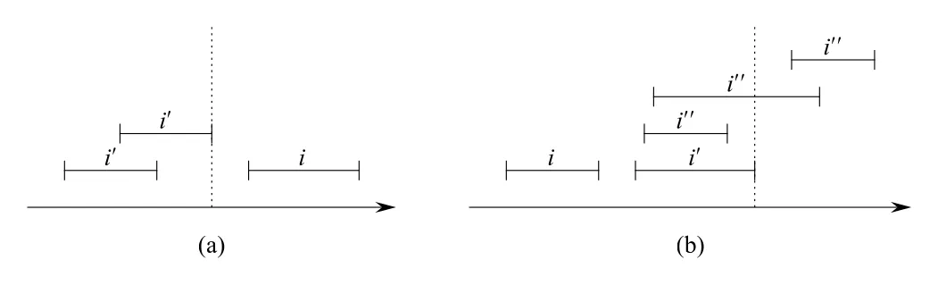Figure 14.5 · PDF p. 373 · INTERVAL-SEARCH가 left/right로 안전하게 이동하는 이유

Right로 가는 경우는 쉽다. x.left == T.nil이거나 x.left.max < i.low이면 left subtree의 모든 interval i'에 대해

i'.high \le x.left.max < i.low

이므로 left subtree에는 query i와 overlap하는 interval이 없다. 따라서 후보가 있다면 right subtree에만 있을 수 있어 right로 가도 안전하다.

Left로 가는 경우가 더 미묘하다. $x.left.max \ge i.low$ 이면 left subtree 안에 high endpoint가 충분히 큰 interval i'가 존재한다. 만약 left subtree에 실제 overlap이 없다면, trichotomy에 의해 이 i'는 query i의 오른쪽에 있어야 한다.

i.high < i'.low

Interval tree는 low endpoint를 key로 쓰므로, right subtree의 모든 interval i''는

i'.low \le i''.low

를 만족한다. 따라서

i.high < i'.low \le i''.low

이고, right subtree의 intervals도 i와 overlap할 수 없다. 그러므로 left subtree에 overlap이 있든 없든, left로 가는 선택은 invariant를 깨지 않는다.

Loop가 $x = T.nil$ 로 끝났다면 현재 subtree에는 overlap interval이 없다. Invariant의 contrapositive에 의해 전체 tree에도 overlap interval이 없으므로 T.nil 반환이 올바르다.

14.3 Exercises에서 남길 포인트

Interval tree용 LEFT-ROTATE에서 max 갱신은 order-statistic tree의 size 갱신과 같은 local pattern이다. Rotation 후 subtree root가 된 y는 이전 x가 대표하던 subtree 전체를 대표하므로 먼저 $y.\max = x.\max$ 로 둘 수 있고, 이후 children이 바뀐 x.max를 max(x.int.high, x.left.max, x.right.max)로 다시 계산한다.

Open intervals를 지원하려면 overlap test의 endpoint inequality를 조정해야 한다. Closed intervals에서는 $i.low \le j.high$ 와 $j.low \le i.high$ 를 쓰지만, open intervals에서는 endpoint가 같은 경우 overlap하지 않을 수 있으므로 strict inequality가 필요하다.

“overlap하는 interval 중 minimum low endpoint를 가진 interval”을 찾는 문제는 단순 INTERVAL-SEARCH보다 강하다. 하나만 찾으면 되는 기본 search와 달리, 더 왼쪽에 있는 overlap 후보를 놓치지 않도록 left subtree 탐색 가능성을 우선 확인하거나 후보를 저장하며 내려가야 한다.

14.3 Exercises에서 이어지는 응용

All overlapping intervals를 나열하는 문제는 INTERVAL-SEARCH를 여러 번 호출하는 방식으로 접근할 수 있다. 단순 방법은 overlap interval을 찾을 때마다 임시로 삭제하고 다시 search를 반복한 뒤 복구하는 것이다. 출력 개수를 k라 하면 각 search/delete/insert가 $O(\lg n)$ 이므로 $O(k \lg n)$ 이고, 전체 intervals를 모두 훑는 naive bound $O(n)$ 과 비교해 $O(\min(n, k \lg n))$ 로 볼 수 있다.

INTERVAL-SEARCH-EXACTLY(T, i)는 low endpoint와 high endpoint가 모두 같은 interval을 찾아야 한다. Low endpoint를 key로 쓰는 기본 interval tree에서는 같은 low endpoint를 가진 intervals가 여러 개 있을 수 있으므로, tie-breaking key를 (low, high) pair로 확장하거나, 같은 low endpoint node에 secondary structure/list를 두는 방식이 필요하다. 목표는 exact match도 $O(\lg n)$ 을 유지하는 것이다.

MIN-GAP 문제는 dynamic set of numbers에서 인접한 두 수의 최소 차이를 유지하는 augmentation 예다. Red-black tree에 각 subtree의 min, max, min-gap을 저장하면 된다.

\begin{aligned} \text{x.min} &= minimum key in subtree rooted at x \\ \text{x.max} &= maximum key in subtree rooted at x \\ x.min_{gap} &= \min(left.min_{gap}, \\ right.min_{gap}, \\ x.key - left.max, \\ right.min - x.key) \end{aligned}

Sentinel에는 적절한 identity 값을 둔다. 이 값들은 node와 children 정보만으로 계산되므로 Theorem 14.1 유형의 augmentation이 가능하고, MIN-GAP(Q)는 root의 min_gap을 읽어 $O(1)$ 에 답할 수 있다. INSERT, DELETE, SEARCH는 red-black tree update와 attribute maintenance를 포함해 $O(\lg n)$ 이다.

Rectangle overlap 문제는 sweep line과 interval tree의 결합으로 이해할 수 있다. Rectangles의 x-coordinates를 events로 정렬하고, sweep line이 왼쪽 edge를 만나면 해당 rectangle의 y-interval을 active interval tree에 삽입한다. 오른쪽 edge를 만나면 삭제한다. 새 rectangle을 삽입하기 전에 active set에서 그 y-interval과 overlap하는 interval이 있는지 INTERVAL-SEARCH로 확인하면, x-range와 y-range가 모두 겹치는 rectangle pair를 찾을 수 있다. Events 정렬 $O(n \lg n)$ , 각 event 처리 $O(\lg n)$ 으로 전체 $O(n \lg n)$ 이다.

Problems for Chapter 14

14-1 Point of maximum overlap

point of maximum overlap은 interval set에서 가장 많은 intervals가 동시에 덮는 point다. 최대 overlap point는 항상 어떤 interval endpoint 중 하나로 잡을 수 있다. Intervals의 내부에서 overlap count는 endpoint를 지나기 전까지 변하지 않기 때문이다.

문제의 hint는 endpoints를 red-black tree에 저장하라는 것이다. Left endpoint에는 +1, right endpoint에는 -1을 부여한다. Inorder order로 endpoints를 훑을 때 prefix sum은 현재 active intervals 수를 뜻한다. 따라서 각 subtree에 다음과 같은 정보를 유지하면 FIND-POM을 빠르게 답할 수 있다.

\begin{aligned} \text{x.sum} &= subtree endpoint values의 합 \\ x.max_{pref} &= subtree inorder prefix sum의 최대값 \\ \text{x.pom} &= max_{pref}를 달성하는 endpoint \end{aligned}

이 역시 subtree-local하게 계산 가능하므로 augmentation theorem의 관점으로 설계할 수 있다. Root의 pom이 point of maximum overlap이다.

14-2 Josephus permutation

Josephus problem은 n명이 원을 이루고 있을 때 매번 m번째 사람을 제거하여 제거 순서를 출력하는 문제다. m이 상수가 아니면 단순 linked list simulation은 각 제거마다 최대 m칸을 걸을 수 있어 비효율적이다.

Order-statistic tree를 쓰면 현재 남아 있는 사람을 rank로 찾고 삭제할 수 있다.

\begin{aligned} \text{current rank r에서 시작} \\ next &= ((r + m - 2) \bmod remaining) + 1 \\ node &= OS-SELECT(T.root, next) \\ \text{output node.key} \\ RB-DELETE(T, node) \end{aligned}

각 round에서 OS-SELECT와 deletion이 $O(\lg n)$ 이므로 전체 $O(n \lg n)$ 에 (n, m)-Josephus permutation을 출력할 수 있다. 이 문제는 order-statistic tree가 단순 selection뿐 아니라 “동적으로 줄어드는 circular rank system”에도 바로 쓰인다는 좋은 예다.

Chapter notes

Interval trees는 computational geometry와 database-style interval query에서 자주 쓰인다. Static interval database에서는 query interval과 overlap하는 $k$ 개 intervals를 $O(k + \lg n)$ 에 enumerate하는 변형도 있다. Chapter 14에서 다룬 동적 interval tree는 red-black tree augmentation을 통해 INSERT, DELETE, INTERVAL-SEARCH를 모두 worst-case $O(\lg n)$ 에 유지하는 쪽에 초점을 둔다.

복잡도

Operation / 구조	Running time	핵심 이유
`OS-SELECT`	$O(\lg n)$	`x.size`로 한 path만 내려감
`OS-RANK`	$O(\lg n)$	parent pointer로 root까지 올라감
order-statistic `INSERT` / `DELETE`	$O(\lg n)$	path update + constant rotations
Theorem 14.1 attribute maintenance	$O(\lg n)$ update 유지	subtree-local dependency가 ancestors로만 전파
`INTERVAL-SEARCH`	$O(\lg n)$	`x.max`로 한 safe path만 탐색
interval tree `INSERT` / `DELETE`	$O(\lg n)$	`x.max`가 local formula로 유지됨
`MIN-GAP` query	$O(1)$	root에 maintained `min_gap` 저장
Josephus permutation with order-statistic tree	$O(n \lg n)$	`n`번 select/delete
rectangle overlap sweep	$O(n \lg n)$	event sorting + interval tree update/search

연결 관계

Chapter 13의 red-black trees는 Chapter 14 augmentation의 underlying balanced tree다.
Chapter 9의 order statistic 개념이 dynamic set으로 확장되어 order-statistic tree가 된다.
Chapter 12의 inorder order와 rank 개념이 OS-SELECT, OS-RANK의 논리 기반이다.
Theorem 14.1은 이후 여러 augmented balanced tree 설계에서 “추가 field가 children 정보로 계산되는가?”라는 체크리스트 역할을 한다.
Interval tree는 computational geometry의 sweep line, rectangle overlap, time interval database 같은 문제와 연결된다.
Josephus permutation은 order-statistic tree의 rank 기반 delete 응용이다.

오해하기 쉬운 내용

Augmentation은 field를 많이 저장하는 것이 아니다. Query에 필요한 정보이면서 update 때 싸게 유지되는 정보를 골라야 한다.
rank를 node마다 직접 저장하는 것은 직관적이지만 update locality가 나쁘다. x.size처럼 subtree-local한 정보가 더 적합하다.
OS-SELECT의 i-r 조정은 right subtree 안에서 rank를 다시 매기기 위한 것이다.
OS-RANK는 node가 right child일 때만 parent와 parent의 left subtree를 더한다.
Interval tree는 interval의 low endpoint를 BST key로 쓰고, high endpoint 정보는 x.max에 요약한다.
$x.\max \ge i.low$ 는 left subtree에 overlap이 반드시 있다는 뜻이 아니라, 있을 가능성을 버리면 안 된다는 뜻이다.
INTERVAL-SEARCH는 overlap interval 하나를 찾는 operation이다. 모든 overlap intervals를 나열하려면 별도 traversal이나 반복 search가 필요하다.
Closed/open interval에 따라 overlap inequality가 달라진다. Endpoint equality를 포함할지 항상 확인해야 한다.

면접 질문

Data structure augmentation의 4단계를 설명하고, order-statistic tree에 각각 대응시켜 보라.
$x.size = x.left.size + x.right.size + 1$ 이 OS-SELECT를 어떻게 가능하게 하는가?
OS-SELECT(x, i)에서 right subtree로 갈 때 왜 i-r을 넘기는가?
OS-RANK(T, x)가 node가 right child일 때만 값을 더하는 이유는 무엇인가?
Rotation 후 order-statistic tree의 size를 어떤 순서로 갱신해야 하는가?
Theorem 14.1의 조건을 말하고, depth가 왜 좋은 augmentation field가 아닌지 설명하라.
Interval overlap 조건을 closed interval 기준으로 정확히 말하라.
Interval tree에서 x.max는 무엇이며, 왜 Theorem 14.1 조건을 만족하는가?
INTERVAL-SEARCH에서 x.left.max < i.low이면 왜 left subtree를 버려도 되는가?
INTERVAL-SEARCH가 left로 가는 경우에도 correctness invariant가 유지되는 이유는 무엇인가?
MIN-GAP을 지원하려면 각 node에 어떤 정보를 유지하면 되는가?
Josephus permutation을 order-statistic tree로 $O(n \lg n)$ 에 출력하는 방법을 설명하라.