개요
Chapter 25는 database application을 “잘 만들었다”에서 한 단계 더 나아가, 실제 운영 환경에서 빠르고 안정적으로 동작하게 만드는 주제를 다룬다. 핵심 흐름은 performance tuning, performance benchmarks, testing/migration 같은 application development issues, standardization, 그리고 distributed directory systems다.
우선순위가 보류인 장이므로 특정 벤더 기능, 표준 이름, 역사적 세부를 길게 암기하기보다 다음 질문에 답할 수 있게 정리한다.
- performance problem을 어디서 찾고, 어느 layer에서 고칠 것인가?
- physical schema, query, logical schema, hardware tuning은 각각 언제 효과적인가?
- benchmark는 왜 필요하고, 왜 단순 숫자 비교만으로 부족한가?
- application testing/migration, standards, LDAP directory system은 database application 개발에서 어떤 위치를 차지하는가?
핵심 개념
| 개념 | 핵심 의미 | 실무적 질문 |
|---|---|---|
performance tuning | schema, query, parameter, hardware 등을 조정해 특정 application 성능을 개선 | bottleneck이 CPU, disk I/O, lock, network, query plan 중 어디인가? |
bottleneck | 전체 성능을 제한하는 한두 component | 병목 아닌 부분을 개선해도 전체 속도는 거의 안 바뀐다 |
queueing system | DB 내부의 CPU, disk, lock, transaction admission을 queue로 모델링 | utilization이 높아질수록 waiting time이 급증한다 |
physical schema tuning | index, clustered index, materialized view 등을 조정 | query는 빨라지지만 update/maintenance cost가 늘 수 있다 |
tuning levels | application, database parameter, hardware 등 여러 계층에서 tuning | 상위 tuning 후 병목이 disk에서 CPU로 이동할 수 있다 |
세부 정리
25.1 Performance Tuning
performance tuning은 특정 application의 성능을 높이기 위해 database-system design의 여러 선택지를 조정하는 일이다. 조정 대상은 넓다. high-level에서는 schema와 transaction design, 중간에서는 buffer size 같은 database parameters, low-level에서는 disk 수나 memory 같은 hardware가 영향을 준다.
중요한 점은 tuning이 “무조건 더 빠른 구성”을 찾는 일이 아니라 “이 workload에서 실제 병목을 줄이는 선택”이라는 것이다. 같은 index도 lookup-heavy workload에는 성능을 올리지만, update-heavy workload에서는 유지 비용 때문에 성능을 떨어뜨릴 수 있다.
25.1.1 Motivation for Tuning
책은 performance tuning이 추상적인 최적화가 아니라 실제 장애와 지연을 고치는 작업임을 여러 사례로 보여준다.
| 증상 | 원인 | tuning/fix |
|---|---|---|
| web application timeout, CPU usage 매우 높음, disk/network usage 낮음 | 큰 relation lookup query가 full relation scan 수행 | lookup attribute에 index 추가 |
| query performance가 매우 나쁨 | nested subqueries가 많고 optimizer가 bad plan 선택 | query를 join 기반으로 rewrite, 즉 decorrelation |
| row를 많이 가져온 뒤 row마다 별도 query 실행 | database round trip이 지나치게 많음 | 필요한 데이터를 한 query로 가져오도록 application/query rewrite |
| light load test에서는 정상, real heavy load에서는 중단 | JDBC connections를 close하지 않아 connection limit 도달 | connection close 보장, connection pooling 사용 |
이 사례들의 공통점은 문제가 live system에서 드러났다는 점이다. test database가 실제보다 작거나 concurrent users 수가 적으면 성능 문제가 숨어 있다가 운영 중 터진다. 따라서 performance testing은 realistic database size와 realistic load에서 수행해야 한다.
connection pooling은 application tuning의 대표 예다. database connection을 transaction마다 열고 닫으면 overhead가 크므로, 열린 connection을 pool에 유지했다가 다음 transaction이 재사용하게 한다. 단, pool을 쓰더라도 connection leak을 방치하면 결국 connection limit에 걸릴 수 있다.
25.1.2 Location of Bottlenecks
대부분의 system은 tuning 전에는 하나 또는 몇 개의 component가 전체 performance를 제한한다. 이를 bottleneck이라고 한다. 어떤 프로그램이 시간의 80%를 작은 loop에서 쓰고 나머지 20%만 다른 코드에서 쓴다면, 나머지 코드를 아무리 빨리 해도 전체 개선은 최대 20%에 가깝다. 반대로 그 loop를 개선하면 전체 성능이 크게 바뀐다.
database system에서는 병목이 단순 CPU loop에만 있지 않다. query execution은 CPU time, disk I/O, network communication, lock waiting을 모두 포함한다. 따라서 tuning의 첫 단계는 다음을 모니터링하는 것이다.
| 관찰 대상 | 찾으려는 병목 |
|---|---|
| operating system monitoring | CPU usage, disk usage, network usage |
| database monitoring | resource-heavy queries, repeated query templates, lock contention |
| query/transaction status | 실행 중인 query, wait state, lock queue |
| workload history | 어떤 SQL statement가 전체 resource를 많이 쓰는지 |
대부분의 DBMS는 performance monitoring용 view, command, stored procedure를 제공한다. 예를 들어 PostgreSQL의 statement/lock monitoring views, MySQL의 show processinfo, SQL Server의 sp_monitor, sp_who, sp_lock 같은 도구가 이 범주다. 특정 제품 이름을 외우는 것이 핵심은 아니고, DBMS 내부 상태를 query 가능한 monitoring surface로 노출한다는 점이 중요하다.
성능 문제는 queueing 관점으로도 이해할 수 있다. transaction은 server process 입장, disk read, CPU cycles, lock acquisition 같은 여러 service를 요청한다. 각 service에는 queue가 있고, small transaction이라도 실제 실행보다 queue waiting에 시간을 더 쓸 수 있다.
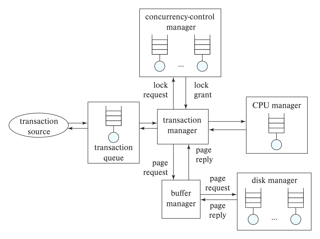 Figure 25.1 · PDF p. 1242 · DBMS 내부에서 transaction, lock, buffer, disk, CPU 요청이 queue를 거치는 구조
Figure 25.1은 database system을 여러 queues의 조합으로 보여준다. concurrency-control manager에는 lockable item마다 queue가 있을 수 있고, disk manager에는 disk별 queue가 있을 수 있다. transaction queue는 동시에 실행 가능한 query task 수보다 요청이 많을 때 admission을 제어한다.
queueing theory의 직관은 강하다. resource utilization이 낮으면 요청이 들어왔을 때 resource가 idle일 가능성이 높아 waiting time이 작다. 하지만 utilization이 100%에 가까워질수록 queue length와 waiting time이 급격히 증가한다. 책은 경험 법칙으로 약 70% utilization은 양호하고, 90%를 넘으면 significant delay를 유발하는 과도한 수준으로 본다.
25.1.3 Tuning Levels
tuning은 database system 내부와 외부 여러 layer에서 일어난다. database 위 application layer에서는 CPU-heavy code block을 profiling해 rewrite하거나, application server parameters를 조정하거나, multiple application servers와 load balancer를 사용해 workload를 나눌 수 있다. web interface 자체도 JavaScript/Ajax 기반으로 바꾸어 responsiveness를 높일 수 있다.
database tuning은 크게 세 level로 나눌 수 있다.
| level | 조정 주체/대상 | 예 |
|---|---|---|
| high level | application developer가 주로 제어 | schema design, indices, transactions, query rewrite |
| database-system parameter level | DBMS별 tunable parameters | buffer size, checkpointing intervals |
| hardware level | physical resource 조정 | SSD/flash storage, disks/RAID, memory, processors |
이 세 level은 독립적이지 않다. query와 physical schema를 고치면 병목이 disk에서 CPU로 옮겨갈 수 있고, 반대로 hardware를 늘려도 query plan이 나쁘면 효과가 제한된다. 일반적으로는 query와 physical schema tuning을 먼저 수행하고, DBMS parameter tuning을 병행한다. 그래도 성능이 부족하면 logical schema와 hardware tuning이 다음 단계가 된다.
25.1.4 Tuning of Physical Schema
physical schema tuning은 application code를 건드리지 않으므로 비교적 disruption이 작다. 대표 대상은 indices, clustered index, materialized views다.
25.1.4.1 Tuning of Indices
query가 병목이면 적절한 index를 만들어 speed up할 수 있다. 반대로 update가 병목이면 index가 너무 많아 update마다 여러 index를 갱신하느라 느릴 수 있으므로 일부 index를 제거하는 것이 도움이 될 수 있다.
index type 선택도 중요하다.
| workload | 적합한 index 선택 |
|---|---|
| range queries가 흔함 | B+ -tree index가 hash index보다 적합 |
| very high write load, relatively low read load | write-optimized LSM tree 계열이 B+ -tree보다 유리할 수 있음 |
| equality lookup 중심 | hash index가 후보가 될 수 있음 |
clustered index 선택도 tuning parameter다. relation은 하나의 physical order만 가질 수 있으므로 clustered index는 relation당 하나만 가능하다. 따라서 가장 많은 queries와 updates에 이득을 주는 index를 clustered index로 선택해야 한다.
대부분의 상용 DBMS는 tuning wizard 또는 physical design advisor를 제공한다. 이 도구들은 과거 query/update history인 workload를 사용해 어떤 index를 만들거나 clustered로 지정했을 때 execution time이 어떻게 바뀔지 추정하고 recommendation을 생성한다.
25.1.4.2 Using Materialized Views
materialized view는 특히 aggregate query를 크게 빠르게 할 수 있다. 예를 들어 department별 total salary를 자주 묻는다면, 매번 instructor를 group-by하고 sum하는 대신 department별 total salary를 저장한 materialized view를 유지할 수 있다.
하지만 materialized view는 공짜가 아니다.
| 비용/선택 | 의미 |
|---|---|
| space overhead | view 결과를 실제로 저장해야 함 |
| maintenance time overhead | base relation update가 view update를 유발 |
| immediate view maintenance | 같은 transaction 안에서 view를 갱신해 consistency는 좋지만 update transaction이 느려짐 |
| deferred view maintenance | 나중에 갱신해 update 부담은 줄지만 view가 일시적으로 inconsistent할 수 있음 |
따라서 materialized view 선택과 view-maintenance policy는 workload를 보고 결정해야 한다. 어떤 queries를 더 빠르게 해야 하는지, 어떤 updates나 queries가 조금 느려져도 되는지를 함께 판단해야 한다.
25.1.4.3 Horizontal Partitioning of Relation Schema
horizontal partitioning은 parallel/distributed storage에서만 쓰이는 것이 아니라 centralized system에서도 query/update 성능 개선에 사용할 수 있다. relation의 tuples를 partitioning attribute 기준으로 여러 partitions에 나누면, predicate가 partitioning attribute를 포함할 때 관련 partitions만 접근할 수 있다.
예를 들어 큰 relation에 date attribute가 있고 대부분의 operations가 최근 몇 달 data에 집중된다면, (year, month)별 partition을 둘 수 있다. date = '2018-06-01' 같은 selection은 해당 date를 포함할 수 있는 partition만 읽고 나머지는 건너뛴다.
partitioning의 성능상 이점은 index에도 이어진다. 전체 relation 하나에 큰 index를 두는 대신 partition마다 separate index를 두면, date range가 주어진 query는 관련 partitions의 작은 index만 lookup한다. index insertion도 전체 relation index보다 작고 빠르며, total data size가 커져도 partition size를 일정 한계 안에 유지하면 query performance degradation을 늦출 수 있다.
trade-off도 명확하다. partitioning attribute에 대한 selection이 없는 query는 모든 partitions를 개별적으로 접근해야 하므로 느려질 수 있다. 따라서 그런 query가 드물고 partition-pruning이 잘 되는 workload에서 유리하다.
DBMS가 내부 partitioning을 지원하지 않아도 비슷한 효과를 흉내낼 수 있다. relation r을 물리적으로 r1, r2, ..., rn으로 나누고, 원래 relation을 다음 view로 정의한다.
optimizer가 각 r_i의 predicate, 예를 들어 date range를 알고 있다면, r에 대한 query 중 partitioning attribute selection이 있는 query를 관련 r_i만 접근하도록 바꿀 수 있다.
25.1.4.4 Automated Tuning of Physical Design
상용 database systems는 index, materialized view, partitioning 같은 physical database design 선택을 돕는 tuning tools를 제공한다. 핵심 입력은 workload, 즉 일정 기간 실행된 queries와 updates의 history다.
automated tuning tool은 보통 다음 흐름으로 동작한다.
| 단계 | 설명 |
|---|---|
| workload collection | 실제 실행된 queries/updates를 수집 |
| workload compression | 같은 형태의 queries/updates를 representative와 weight로 압축 |
| candidate generation | 유용할 수 있는 indices, materialized views, partitions 후보 생성 |
| optimizer cost estimation | query optimizer를 사용해 후보별 cost/benefit 추정 |
| heuristic search | 가능한 조합이 너무 많으므로 greedy 등 heuristic으로 선택 |
| recommendation | DBA에게 index/view/partition 생성 또는 삭제 권고 |
workload compression은 필수다. 실제 workload는 매우 클 수 있으므로, 같은 form의 update를 하나의 representative update와 occurrence count로 압축하고, 드물고 비용도 낮은 queries는 제외할 수 있다. expensive queries를 우선 대상으로 삼는다.
candidate 조합은 exponential하게 많아질 수 있다. index와 materialized view 후보가 많고, 그 부분집합마다 설계안이 되기 때문이다. 따라서 exhaustive search는 실용적이지 않다. 흔한 방식은 greedy heuristic이다. 각 index/view 후보의 benefit 또는 benefit per unit space를 optimizer cost estimation으로 계산하고, 가장 큰 이득을 주는 후보를 선택한다. 하나를 선택하면 다른 후보의 marginal benefit이 바뀌므로 다시 계산하고 다음 후보를 고른다. disk space가 소진되거나 maintenance cost가 query benefit보다 커질 때 멈춘다.
자동 tuning에는 위험도 있다. 새 index를 만들면 optimizer가 잘못된 cost estimate 때문에 이전보다 느린 plan을 선택할 수 있다. 일부 systems는 query performance를 monitoring하다가 성능이 나빠지면 이전의 “last good plan”을 강제하는 방식으로 이런 위험을 줄인다. 핵심은 physical design 자동화도 결국 optimizer statistics와 runtime monitoring의 품질에 의존한다는 점이다.
25.1.5 Tuning of Queries
application performance는 query rewrite 또는 application이 database에 query를 보내는 방식을 바꾸는 것만으로도 크게 개선될 수 있다.
25.1.5.1 Tuning of Query Plans
현대 optimizer는 예전보다 강하지만, 여전히 bad plan을 고를 수 있다. tuning 전에 먼저 실제 query plan을 확인해야 한다. 대부분의 DBMS는 explain command를 제공한다. explain은 사용 중인 plan, optimizer가 사용한 statistics, plan 각 부분의 estimated cost를 보여준다. 일부 variant는 query를 실제 실행해 actual tuple counts와 execution time도 보여준다.
bad plan의 대표 원인은 incorrect statistics다. optimizer가 join 대상 relation을 작게 추정하면 nested loops join을 선택할 수 있는데, 실제 relation이 크면 매우 비효율적이다. 이상적으로는 relation update 때마다 statistics도 갱신되어야 하지만 update overhead가 크므로, DBMS는 보통 주기적으로 갱신하거나 administrator가 analyze 같은 command로 재계산하게 한다. data load 직후, 또는 많은 inserts/deletes 이후에는 statistics 갱신이 특히 중요하다.
필요한 index가 없는 것도 query 성능 저하의 원인이다. 큰 relation에서 predicate로 소수 rows만 가져오는 query에는 predicate attribute index가 중요하다. join attribute index도 매우 유용하다. primary key index는 selection과 join 모두에 사용될 수 있다.
nested subquery도 주의할 대상이다. optimizer가 decorrelation에 실패하면 subquery가 반복 실행되어 random I/O가 크게 증가할 수 있다. query를 manual rewrite하여 joins 같은 set-oriented operations로 바꾸면 random I/O를 줄일 수 있다.
25.1.5.2 Improving Set Orientation
application에서 같은 SQL query를 parameter만 바꿔 반복 호출하면 communication overhead와 server-side processing overhead가 반복된다. set-oriented SQL로 묶으면 한 번의 scan과 한 번의 result transfer로 처리할 수 있다.
예를 들어 application이 각 department마다 다음 query를 반복 실행한다고 하자.
select sum(salary)
from instructor
where dept_name = ?;dept_name에 clustered index가 없으면 department마다 relation scan이 발생할 수 있고, index가 있어도 department마다 random I/O가 발생한다. 이를 다음처럼 한 query로 바꾸면 instructor relation을 한 번 scan하고 결과를 client가 순회하면 된다.
select dept_name, sum(salary)
from instructor
group by dept_name;
이런 변경의 본질은 row-by-row 또는 parameter-by-parameter access를 set-oriented access로 바꾸는 것이다.
JDBC의 batch update도 같은 맥락이다. 여러 inserts를 개별 communication round로 보내지 않고 batch에 모아 한 번에 보낸다.
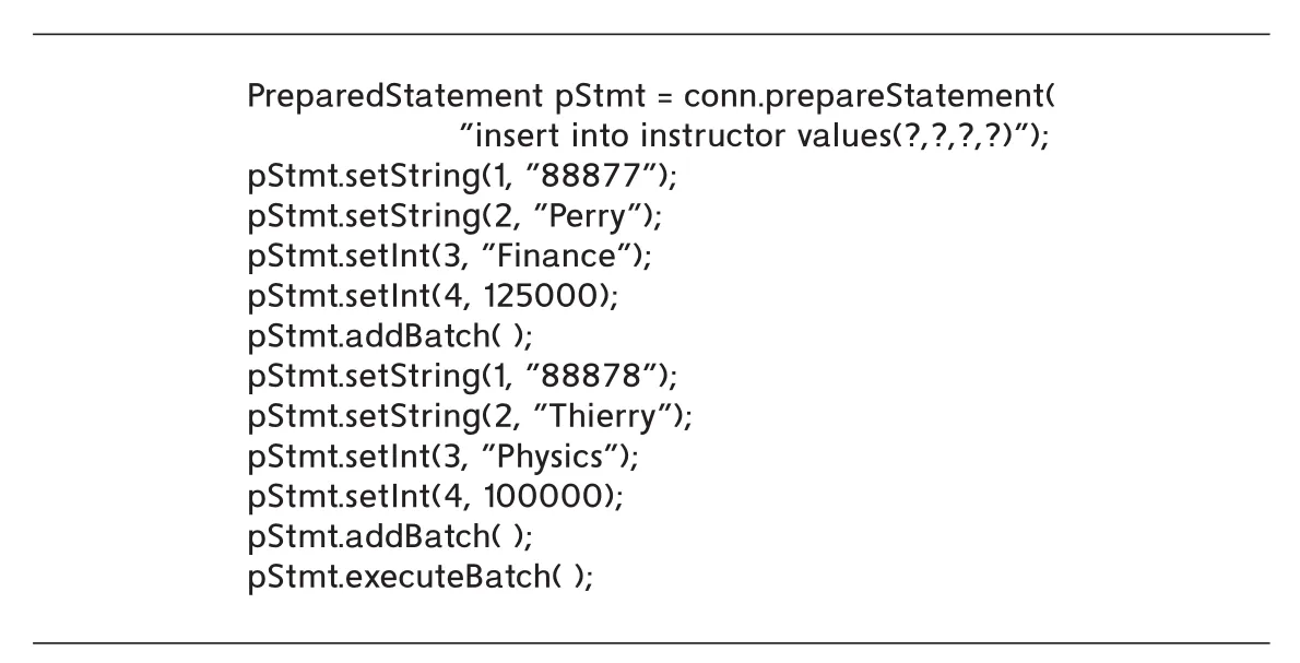 Figure 25.2 · PDF p. 1250 · JDBC PreparedStatement의 addBatch/executeBatch를 이용한 batch update
Figure 25.2의 코드는 addBatch()로 여러 insert parameter sets를 쌓고, executeBatch() 시점에 database와 한 번 communication한다. batch update는 network round trip을 줄이고, DBMS가 여러 inserts를 한꺼번에 처리할 기회를 준다.
stored procedures도 client-server communication과 SQL compilation cost를 줄이는 데 쓰인다. queries를 server-side procedure로 저장하고 precompiled 형태로 둘 수 있으며, client는 여러 query를 직접 보내는 대신 stored procedure를 호출한다.
25.1.5.3 Tuning of Bulk Loads and Updates
large volume data를 database에 넣는 bulk load에서 tuple마다 별도 SQL insert를 수행하면 성능이 매우 나쁘다. 이유는 SQL parsing overhead뿐 아니라 integrity constraint checks와 index updates가 tuple마다 따로 수행되어 random I/O가 많아지기 때문이다. 큰 batch로 처리하면 constraint checking과 index maintenance를 set-oriented 방식으로 수행할 수 있어 한 자릿수 이상, 때로는 order-of-magnitude 개선이 가능하다.
대부분의 DBMS는 bulk import와 bulk export utility를 제공한다. 입력/출력 format은 comma-separated values(CSV), tab-separated values(TSV), database-specific binary format, XML 등이 될 수 있다. 유틸리티 이름은 DBMS마다 다르므로 이름 암기보다 역할을 이해하면 된다. 핵심은 file에서 data를 읽고 integrity constraint checking과 index maintenance를 효율적으로 수행한다는 점이다.
bulk update에서는 merge construct가 유용하다. master table에 batch updates를 반영해야 하는 상황을 생각하자. 예를 들어 funds_received(dept_name, amount)의 amount를 department.budget에 더해야 한다면, SQL:2003의 merge는 matching record를 update하고, 필요하면 unmatched record를 insert할 수 있다.
merge into department as A
using (select * from funds_received) as F
  on (A.dept_name = F.dept_name)
when matched then
  update set budget = budget + F.amount;
when not matched then clause를 추가하면 master relation에 없는 새 records를 insert할 수 있다. 즉 merge는 batch로 들어온 변경분을 기존 relation과 맞춰 update/insert하는 set-oriented construct다. 모든 SQL implementation이 merge를 지원하는 것은 아니므로 실제 사용은 system manual 확인이 필요하다.
25.1.6 Tuning of the Logical Schema
logical schema도 성능 tuning 대상이 될 수 있다. 예를 들어 course(course_id, title, dept_name, credits)에서 course_id가 key이면, 정규형(BCNF/3NF) 제약을 지키면서 다음처럼 vertical partitioning할 수 있다.
course_credit(course_id, credits)
course_title_dept(course_id, title, dept_name)
두 표현은 course_id가 key이므로 논리적으로 equivalent하다. 하지만 access pattern에 따라 performance characteristics가 달라진다. 대부분의 access가 course_id와 credits만 읽는다면 작은 course_credit relation만 접근하면 되어 I/O가 줄어든다. 반대로 title, dept_name, credits를 함께 자주 읽는 workload라면 join cost가 늘 수 있다.
column store는 vertical partitioning을 극단까지 밀어붙인 저장 방식이다. 각 attribute, 즉 column을 별도 file에 저장한다. row reconstruction은 필요한 columns의 i번째 entry들을 결합하면 되므로 primary key를 매 column마다 반복할 필요가 없다. column stores는 data-warehouse applications에서 I/O 감소, cache performance 개선, compression 이득, CPU vector-processing 활용 때문에 좋은 성능을 낼 수 있다.
logical schema tuning의 더 공격적인 방식은 denormalized relation을 저장하는 것이다. 예를 들어 instructor와 department의 join 결과를 미리 저장하면 instructor name과 building을 가져오는 query는 join 없이 빨라진다. 하지만 department building이나 budget이 바뀔 때 instructor별로 반복 저장된 redundant data를 모두 consistent하게 유지해야 한다. 이 consistency 유지 부담을 programmer가 직접 지는 것이 denormalization의 위험이다.
materialized views는 denormalized relation과 비슷한 query-speed benefit을 주면서 redundant data consistency 관리를 DBMS가 맡는다는 장점이 있다. DBMS가 materialized view를 지원한다면, 직접 denormalized relation을 관리하는 것보다 materialized view가 더 안전한 선택일 수 있다.
join을 materialize하지 않고도 join cost를 줄이는 방법은 join에서 match될 records를 같은 disk page에 모으는 clustered file organization이다. 이 방식은 storage layout을 통해 join locality를 높인다.
25.1.7 Tuning of Concurrent Transactions
concurrent transactions의 성능 문제는 주로 lock contention에서 나온다. 책은 read-write contention과 write-write contention을 나누어 설명한다.
read-write contention의 전형적 예는 banking database에서 낮에는 작은 update transactions가 계속 실행되고, 동시에 branch statistics를 계산하는 large query가 relation scan을 수행하는 상황이다. large query가 locks를 오래 잡으면 updates가 막혀 전체 system performance가 급격히 나빠질 수 있다.
가능하면 large read queries에는 snapshot isolation을 사용하는 것이 좋다. snapshot isolation은 query가 data snapshot을 읽는 동안 updates가 계속 진행될 수 있게 하므로 read-write lock contention을 줄인다. snapshot isolation을 사용할 수 없다면 large query를 updates가 적은 시간에 실행하거나, application semantics가 허용한다면 read committed 같은 weaker consistency level로 approximate/inconsistent result를 받아들일 수 있다.
write-write contention은 자주 update되는 data item, 즉 update hot spot에서 발생한다. 예를 들어 새 tuple에 unique identifier를 부여하기 위해 database tuple 안의 sequence counter를 읽고 증가시키는 방식은, inserts가 많을 때 그 counter tuple이 hot spot이 된다.
이 문제를 줄이기 위해 DBMS는 보통 sequence construct나 identity attribute를 제공한다. 이들은 non-two-phase lock release와 특수한 undo logging 처리를 통해 sequence counter update가 transaction abort 때 rollback되지 않게 한다. 그래야 concurrent transaction이 이미 받은 sequence number와 충돌하지 않는다.
하지만 이 설계는 gaps in sequence numbers를 만들 수 있다. transaction이 sequence number 1002를 받은 뒤 abort하면, 1001과 1003은 있지만 1002는 없는 상태가 된다. 일반 surrogate key에는 괜찮지만, bill number나 receipt number처럼 gap이 법적/업무적으로 허용되지 않는 application에는 DBMS sequence/identity를 그대로 쓰면 안 된다. 이런 경우에는 normal tuple에 저장된 sequence counter를 two-phase locking으로 다루어 abort 시 counter value가 복구되도록 해야 한다.
long update transaction도 성능 문제를 만든다. updates가 많으면 system log가 transaction 완료 전 가득 찰 수 있고, 오래 실행되는 update transaction은 old log deletion을 막아 log space를 압박할 수 있다. 이를 줄이기 위해 DBMS가 transaction당 update 수를 제한하거나, application이 큰 update를 여러 minibatch transactions로 나눌 수 있다.
minibatch는 조심해야 한다. 하나의 큰 transaction과 의미가 같지 않을 수 있고, failure가 발생하면 일부 minibatch만 commit되어 partial update 상태가 될 수 있다. recovery 후 남은 minibatch를 계속 실행하는 절차가 필요하다.
long transaction은 lock table도 가득 차게 할 수 있다. 많은 tuple locks를 잡는 transaction에 대해 일부 DBMS는 lock escalation을 수행한다. 즉 tuple locks를 page locks 또는 relation locks로 승격해 lock table entries를 줄인다. multiple-granularity locking 관점에서는 coarse-grained lock을 얻으면 finer-grained locks를 기록할 필요가 줄어든다.
25.1.8 Tuning of Hardware
hardware bottleneck은 memory, I/O, CPU, network capacity에서 생길 수 있다. 이 절의 핵심은 transaction processing에서 disk random I/O가 throughput을 쉽게 제한한다는 점이다.
예를 들어 hard disk가 평균 access time 약 10ms라면 4KB random I/O를 초당 100개보다 조금 적게 처리한다. transaction 하나가 I/O 두 번만 필요해도 disk 하나는 최대 약 50 transactions/sec 정도밖에 지원하지 못한다. SSD는 random I/O를 훨씬 많이 처리하지만 같은 capacity당 비용이 높다.
throughput을 높이는 방법은 크게 세 가지다.
| 방법 | 효과 | 주의점 |
|---|---|---|
| hard disk를 SSD로 교체 | random I/O capacity 대폭 증가 | capacity당 비용 증가 |
| disks 수 증가/striping | I/O parallelism 증가 | skew가 있으면 일부 disk가 병목 |
| memory 증가 | frequently used pages를 cache하여 disk I/O 감소 | infrequently used data를 cache하면 낭비 |
memory와 disk 사이의 경제적 trade-off를 판단하는 대표 직관이 five minute rule 계열이다. 어떤 page를 memory에 두는 비용과 disk에서 읽는 비용 절감을 비교해, page가 일정 시간보다 자주 접근되면 memory에 cache하는 것이 이득이라는 규칙이다.
책의 일반식은 다음처럼 볼 수 있다. 초당 1 I/O를 줄이는 가치를 disk 가격과 disk access/sec로 계산하고, page 하나를 memory에 두는 비용과 같아지는 access interval m을 찾는다.
이 식의 숫자는 hardware 가격과 성능에 따라 시대별로 달라진다. 과거에는 4KB page 기준 “5분보다 자주 접근되면 memory cache가 이득”이라는 five minute rule이 널리 쓰였다. 책의 2018년 기준 예시는 hard disk random access에서는 몇 시간 단위, SSD와 비교하면 몇 분 단위로 바뀐다. 핵심은 특정 숫자가 아니라, random I/O cost와 memory cost의 상대 변화에 따라 cache decision threshold가 달라진다는 점이다.
sequential access에서는 상황이 다르다. 한 번에 많은 pages를 읽을 수 있으므로 page당 I/O cost가 낮고, sequentially accessed data는 아주 자주 쓰이지 않는 한 memory cache 이득이 작다. 반대로 response time이 매우 중요한 application은 cost 계산상 이득이 작아도 data를 memory에 둘 수 있다.
flash-as-buffer approach는 SSD/flash storage를 persistent buffer로 사용한다. 각 block은 disk에 permanent location을 갖지만, 자주 쓰이면 disk 대신 flash에 머문다. flash가 가득 차면 자주 쓰이지 않는 block을 evict하고, dirty block이면 disk로 flush한다. DBMS가 직접 SSD와 disk를 모두 볼 수 있다면 tablespace를 이용해 frequently used relations/indices를 flash storage에 배치할 수도 있다.
RAID 선택도 workload에 의존한다. RAID 5는 random write 하나에 2 reads와 2 writes가 필요하므로 random update가 많은 workload에서는 RAID 1보다 느릴 수 있다. 초당 random reads가 r, random writes가 w라면 대략 다음 I/O 부담을 비교할 수 있다.
| RAID | I/O operations/sec 부담 |
|---|---|
RAID 5 | r + 4w |
RAID 1 | r + 2w |
update rate, 특히 random update rate가 크면 RAID 5의 storage efficiency보다 write penalty가 더 큰 문제가 된다. RAID 5는 data size가 매우 크고 random update rate가 낮은 경우에 더 적합하다.
25.1.9 Performance Simulation
database system을 설치하기 전에도 performance-simulation model을 만들어 성능을 추정할 수 있다. Figure 25.1의 CPU, disk, buffer, concurrency control 같은 services를 simulation model의 service로 보고, 각 service에는 service time과 queue를 둔다.
transaction은 여러 service requests의 sequence다. requests는 도착 순서대로 queue에 들어가고, 각 service의 policy, 예를 들어 first come, first served에 따라 처리된다. CPU와 disks 같은 subsystems는 실제 system처럼 병렬로 동작한다고 모델링한다.
simulation model을 만든 뒤에는 simulated transactions arrival rate를 바꿔 load condition별 behavior를 실험할 수 있다. 또 service time이나 system parameters를 바꿔 어떤 component가 performance에 민감한지 확인할 수 있다. 즉 performance simulation은 실제 hardware를 사거나 설치하기 전에 bottleneck과 tuning parameter의 효과를 탐색하는 도구다.
25.2 Performance Benchmarks
performance benchmarks는 software system 성능을 정량화하기 위한 standardized tasks의 suite다. database servers가 기능적으로 표준화될수록 제품 차이는 performance에서 드러나기 쉬운데, 단일 task 하나로는 system 성능을 대표하기 어렵다. 어떤 DBMS는 특정 transaction에는 빠르지만 다른 transaction에는 느릴 수 있기 때문이다.
25.2.1 Suites of Tasks
benchmark는 여러 task의 성능을 조합해야 하며, 조합 방식이 중요하다. throughput을 단순 산술 평균하면 잘못된 결론이 나올 수 있다.
예를 들어 system A가 T1 = 99 TPS, T2 = 1 TPS이고 system B가 T1 = 50 TPS, T2 = 50 TPS라고 하자. 산술 평균은 둘 다 50 TPS지만, workload가 T1/T2를 50개씩 실행한다면 A는 T2 때문에 약 50.5초가 걸리고, B는 약 2초면 끝난다. 따라서 mixed workload에서는 transaction type별 throughput 평균이 아니라 workload completion time을 기준으로 봐야 한다.
동일 확률로 transaction types가 등장하고 서로 간섭이 없다는 조건에서는 throughputs의 harmonic mean이 올바른 평균이다.
이 예시에서 A의 harmonic mean은 약 1.98 TPS, B는 50 TPS다. 즉 산술 평균으로는 같은 성능처럼 보이지만 실제 mixed workload에서는 B가 훨씬 빠르다.
25.2.2 Database-Application Classes
database application은 크게 online transaction processing (OLTP)와 decision support, 즉 online analytical processing (OLAP) 계열로 나눌 수 있다.
| class | 요구사항 | 대표 tuning 초점 |
|---|---|---|
OLTP | 많은 짧은 update transactions, high concurrency | commit processing, lock/concurrency, short response time |
OLAP/decision support | 큰 scan, aggregation, complex queries | query evaluation algorithms, query optimization, parallelism |
실제 application은 OLTP와 decision support 요구를 섞어 가진다. 따라서 “어느 DBMS가 최고인가”는 application의 workload mix에 따라 달라진다. 단, OLTP throughput과 decision-support throughput을 따로 측정한 뒤 harmonic mean을 취하는 것도 조심해야 한다. long-running decision-support transaction이 locks를 잡아 update transactions를 막는 식의 interference가 있으면 단순 조합이 실제 성능을 반영하지 못한다.
25.2.3 The TPC Benchmarks
Transaction Processing Performance Council (TPC)는 database systems용 benchmark standards를 정의한다. TPC benchmark는 relations, tuple sizes, relation sizes, transaction mix, response time bound, price/performance metric, external audit 같은 조건을 매우 구체적으로 정한다. benchmark 수치를 주장하려면 ACID properties를 포함해 benchmark 정의를 충실히 따랐음을 외부 audit으로 확인받아야 한다.
TPC 계열은 benchmark가 workload 성격에 따라 달라져야 함을 잘 보여준다.
| benchmark | 목적/성격 |
|---|---|
TPC-A, TPC-B | 초기 bank teller/backend DB 성능 모델, 현재는 사용되지 않음 |
TPC-C | order-entry environment를 모델링한 OLTP benchmark, 여전히 널리 사용 |
TPC-E | brokerage firm 모델 기반 OLTP benchmark |
TPC-D | decision-support queries용 benchmark, sales/distribution schema와 17 SQL queries |
TPC-H | ad hoc decision-support benchmark, materialized views/redundant information 금지, primary/foreign key index만 허용 |
TPC-R | reporting 성격, materialized views 허용, 현재는 사용되지 않음 |
TPC-DS | retail supplier의 decision-support workload, ad hoc querying/reporting과 data maintenance 포함 |
OLTP benchmark를 decision-support 성능 지표로 쓰면 안 된다. TPC-A/B/C가 transaction-processing workload를 재는 반면, TPC-D/H/DS는 large analytical queries, aggregation, nested queries, updates/data maintenance 등을 다룬다.
TPC-H는 “queries를 미리 알 수 없는 ad hoc querying”을 모델링하므로 materialized views와 redundant information을 금지한다. 반대로 reporting workload처럼 queries가 미리 알려져 있으면 materialized views를 신중히 선택해 queries를 빠르게 할 수 있지만, 그 maintenance overhead도 benchmark에 반영해야 한다.
TPC-H와 TPC-DS의 decision-support 성능 측정은 두 축을 사용한다.
| metric | 의미 |
|---|---|
| power test | queries/updates를 하나씩 sequential하게 실행해 single-stream 성능 측정 |
| throughput test | multiple streams를 parallel하게 실행하고 update stream도 포함 |
| composite query per hour | power와 throughput metrics의 곱의 square root |
| composite price/performance | system price를 composite metric으로 나눈 값 |
benchmark를 읽을 때는 단순히 “TPS가 높다”만 볼 것이 아니라, workload class, response time bound, data scale, allowed physical design, price/performance, audit 조건을 함께 봐야 한다.
25.3 Other Issues in Application Development
이 절은 database application 개발에서 성능 외에도 반드시 다뤄야 하는 두 문제, testing applications와 application migration을 다룬다.
25.3.1 Testing Applications
program testing은 test cases의 모음인 test suite를 설계하는 일이다. 프로그램은 계속 바뀌며, 변경의 의도치 않은 결과로 기존 동작이 깨지는 program regression이 생길 수 있다. 따라서 매 변경 후 사람이 수동으로 확인하는 대신, test case마다 expected output을 저장해 두고 자동으로 비교하는 regression testing이 필요하다.
database application의 test case는 보통 두 부분으로 구성된다.
| test case 구성요소 | 의미 |
|---|---|
| database state | test 시작 시점의 relation contents |
| application input | 특정 interface에 주는 입력 |
SQL query bug는 미묘하다. 예를 들어 개발자가 outer join을 써야 하는데 natural join을 썼다면, test database에 matching tuple이 모두 존재하는 경우 두 query 결과가 같아 bug가 드러나지 않는다. 그래서 test database는 흔한 오류를 드러내도록 설계되어야 한다.
이 문맥에서 mutant는 원래 query/program에 작은 변경을 가한 오류 후보를 뜻한다. 어떤 test case가 intended query와 mutant query에서 다른 output을 만들면 그 test case가 mutant를 kill한다고 말한다. 좋은 test suite는 흔한 mutants를 많이 kill해야 한다.
update를 수행하는 test case는 화면 output만 확인해서는 부족하다. test 실행 후 database state가 expected state와 일치하는지도 확인해야 한다. 또한 여러 test cases가 같은 database state를 공유한다면, update test가 끝난 뒤 database를 original state로 restore해야 한다. 그렇지 않으면 뒤의 test가 잘못 실패한 것으로 보고될 수 있다.
performance testing도 testing의 일부다. 이때 test database는 실제 production database와 비슷한 size여야 한다. 기존 data를 쓸 수 없거나 민감한 data가 포함되어 있으면 test database를 생성하거나, real database copy의 sensitive values를 obfuscation해야 한다. primary key 값을 obfuscate하면 references도 함께 바꿔야 하고, date of birth처럼 application logic에 영향을 주는 값은 완전 random replacement보다 작은 random perturbation이 적합할 수 있다.
25.3.2 Application Migration
legacy systems는 오래된 technology로 만들어졌지만 여전히 운영 중인 application systems다. 교체 비용과 risk가 크기 때문에 obsolete 상태여도 계속 사용된다. legacy system은 network/hierarchical data model, Cobol, file system 기반일 수 있고, critical applications와 valuable data를 담고 있을 수 있다.
legacy migration이 어려운 이유는 다음과 같다.
| 어려움 | 설명 |
|---|---|
| code size | 수백만 lines, 수십 년에 걸친 개발 |
| data migration | 새 application은 완전히 다른 schema를 쓸 수 있음 |
| retraining | 많은 사용자가 새 interface를 배워야 함 |
| no disruption requirement | switchover 동안 critical transactions가 멈추면 안 됨 |
| hidden design knowledge | schema/system design 문서가 부족할 수 있음 |
교체 대신 상호운용을 선택할 수도 있다. 이때 legacy system 위에 wrapper layer를 두어 legacy system이 relational database처럼 보이게 만들 수 있다. wrapper는 ODBC, OLE-DB 같은 interconnection standards를 제공하고, relational queries/updates를 legacy system의 query/update로 변환한다.
새 system으로 교체할 때는 reverse engineering과 re-engineering이 중요하다. reverse engineering은 legacy code를 분석해 E-R model이나 object-oriented data model 같은 high-level schema/design을 복원하는 과정이다. re-engineering은 그 분석을 바탕으로 더 나은 새 system을 설계하고 구현하는 전체 과정이다.
전환 방식에는 두 극단이 있다.
| approach | 의미 | 위험/비용 |
|---|---|---|
big-bang approach | 어느 시점에 old system에서 new system으로 급격히 전환 | 사용자 미숙, 미발견 bug/performance issue가 큰 손실로 이어질 수 있음 |
chicken-little approach | legacy functionality를 점진적으로 교체 | wrapper와 coexistence 때문에 development cost 증가 |
mission-critical system에서는 big-bang switchover 실패가 치명적일 수 있다. chicken-little approach는 비용이 더 들지만, new UI와 old backend를 결합하거나, legacy와 분리 가능한 일부 기능부터 새 system을 쓰는 식으로 risk를 낮춘다.
25.4 Standardization
standards는 software system의 interface를 정의한다. programming language의 syntax/semantics, API functions, data model, database connectivity protocol 모두 표준화 대상이 될 수 있다. database systems는 여러 독립 component가 함께 동작해야 하므로 standards가 특히 중요하다.
standard에는 여러 성격이 있다.
| 종류 | 의미 |
|---|---|
formal standards | ISO, ANSI, IEEE, industry group처럼 공개 절차를 거쳐 만든 표준 |
de facto standards | 공식 절차 없이 dominant product나 관행이 사실상 표준이 된 것 |
anticipatory standards | 시장보다 앞서 features를 정의하고 vendors가 구현하도록 이끄는 표준 |
reactionary standards | 이미 vendors가 구현했거나 de facto가 된 features를 나중에 표준화 |
표준은 한 번 정하면 끝이 아니다. 구현과 사용 경험을 통해 shortcomings와 new requirements가 드러나고, committee discussion, proposal, public review, vote를 거쳐 새 version이 나온다.
25.4.1 SQL Standards
SQL은 가장 널리 쓰이는 query language이므로 ANSI/ISO와 database vendors가 오랫동안 표준화해 왔다. SQL-86, SQL-89, SQL-92, SQL:1999, SQL:2003, SQL:2006, SQL:2008, SQL:2011, SQL:2016처럼 버전이 이어졌다.
세부 연도 암기보다 중요한 점은 SQL standard가 기능 확장의 기록이라는 것이다. 예를 들어 SQL:2011은 temporal extensions, period 기반 primary key/update/delete, window construct 확장, fetch clause 등을 포함했고, SQL:2016은 JSON support와 listagg 같은 aggregate feature를 추가했다.
현실적으로는 표준 feature를 모든 DBMS가 똑같이 지원하지 않는다. 새 feature는 일부 DBMS만 지원할 수 있고, 반대로 각 DBMS는 표준 밖의 proprietary features를 제공하기도 한다.
25.4.2 Database Connectivity Standards
ODBC는 client applications와 database systems 사이 communication을 위한 널리 쓰이는 standard다. 여러 언어에서 API를 정의한다. JDBC는 Java applications와 databases 사이 communication 표준으로, ODBC와 유사한 기능을 제공한다.
ODBC API는 CLI, SQL syntax definition, CLI call sequence 규칙, conformance levels를 정의한다. core level은 database connect, SQL prepare/execute, result/status retrieval, transaction management를 포함한다. 더 높은 level은 catalog retrieval, parameter arrays, 더 자세한 catalog information 등을 요구한다.
ODBC는 client가 여러 data sources에 동시에 연결하고 전환할 수 있게 하지만, 각 data source의 transaction은 독립적이다. 즉 ODBC 자체는 two-phase commit을 지원하지 않는다.
distributed transaction에는 X/Open XA standards가 더 직접적이다. XA는 transaction begin, commit, abort, prepare-to-commit 같은 transaction-management primitives를 정의한다. transaction manager는 이 primitives를 호출해 two-phase commit으로 distributed transaction의 global consistency를 보장할 수 있다. XA는 data model과 client-database data interface에 독립적이므로 relational database와 object-oriented database를 한 transaction 안에서 조합하는 환경에도 적용될 수 있다.
relational database가 아닌 data sources도 있다. flat files, email stores 같은 nondatabase sources를 대상으로 Microsoft OLE-DB, ADO, ADO.NET 같은 APIs가 등장했다. 이들은 connection, session, command execution, result rowset retrieval 같은 공통 access pattern을 제공한다.
25.4.3 Object Database Standards
object-oriented database(OODB) 표준화는 주로 OODB vendors가 추진했다. ODMG는 OODB data model과 language interfaces를 표준화하려 했지만 현재는 active하지 않다. JDO는 Java에 persistence를 더하기 위한 표준이다. 여러 object database 관련 표준 시도는 있었지만 널리 채택되지 않았고, 현재는 드물게 쓰인다.
반면 object-relational mapping (ORM)은 널리 쓰인다. ORM은 backend에 relational database를 두고 programmer에게 object-based API를 제공한다. Hibernate(Java), Django data layer(Python)가 대표적이다. 다만 ORM 영역에도 널리 받아들여진 formal standard는 없다.
25.5 Distributed Directory Systems
directory는 persons 같은 object class에 대한 정보를 listing하고, browse/search를 가능하게 하는 system이다. 조직의 employee name, designation, employee-id, address, email, phone number 같은 정보를 공유하는 데 쓰인다.
directory는 단순 검색뿐 아니라 authentication/authorization 기반이 될 수 있다. 여러 applications가 하나의 common directory service를 사용해 users를 authenticate하고, user category와 authorization information을 공유하면 application마다 별도 user database를 유지하지 않아도 된다.
25.5.1 Directory Access Protocols
directory information은 web interface로 사람에게 제공할 수 있지만, programs도 directory에 접근해야 한다. 이를 위해 directory access protocol이 필요하다. 가장 널리 쓰이는 protocol은 LDAP (Lightweight Directory Access Protocol)이다.
directory data도 relational database에 저장하고 JDBC/ODBC로 접근할 수 있는데, 왜 별도 protocol이 필요한가? 핵심 이유는 두 가지다.
| 이유 | 설명 |
|---|---|
| limited access에 맞춘 단순 protocol | directory workload는 일반 DB query보다 단순한 browse/search 중심 |
| hierarchical naming | file system path처럼 object를 계층적으로 이름 붙여 distributed directory servers를 통합 |
hierarchical naming은 site autonomy와 distribution에 특히 유리하다. 예를 들어 한 directory server는 Murray Hill의 Bell Labs employees, 다른 server는 Bangalore employees를 담당할 수 있고, directory system은 query를 적절한 site로 자동 forward할 수 있다.
25.5.2 LDAP: Lightweight Directory Access Protocol
directory system은 보통 여러 clients와 하나 이상의 servers로 구현된다. directory access protocols는 client-server communication API뿐 아니라 data model과 access control도 정의한다. X.500은 ISO의 directory access protocol이지만 복잡해서 널리 쓰이지 않았고, LDAP는 X.500의 많은 기능을 더 낮은 complexity로 제공한다.
25.5.2.1 LDAP Data Model
LDAP directory는 entries를 저장한다. 각 entry는 unique identifier인 distinguished name (DN)을 가져야 한다. DN은 여러 relative distinguished names (RDNs)의 sequence로 구성된다.
예:
cn=Silberschatz, ou=Computer Science, o=Yale University, c=USA여기서 cn은 common name, ou는 organizational unit, o는 organization, c는 country를 나타낸다. DN components의 순서는 file path와 반대로 보일 수 있는데, postal address order처럼 person에서 organization/country 방향으로 나열된다.
LDAP entry는 attributes를 가진다. LDAP attributes는 relational model과 달리 기본적으로 multivalued다. 따라서 한 entry에 여러 telephone numbers나 addresses를 저장할 수 있다. LDAP는 binary, string, time, telephone number, PostalAddress 같은 types를 제공한다.
LDAP는 object classes도 정의할 수 있다. object class는 attribute names와 types를 가진다. inheritance를 사용할 수 있고, entry는 하나 이상의 object classes에 속할 수 있다. 반드시 하나의 most-specific class만 가져야 하는 것은 아니다.
entries는 DN에 따라 directory information tree (DIT)로 조직된다. leaf entries는 보통 specific objects를 나타내고, internal nodes는 organizational unit, organization, country 같은 grouping objects를 나타낸다. entry 자체에 전체 DN을 저장하지 않아도, DIT를 위로 traverse하며 RDN=value components를 모아 full DN을 생성할 수 있다.
entry가 둘 이상의 DN을 가져야 할 수도 있다. 예를 들어 한 사람이 여러 organizations에 속하면, DIT의 leaf level에 다른 branch의 entry를 가리키는 alias를 둘 수 있다.
25.5.2.2 Data Manipulation
LDAP는 SQL처럼 별도의 data-definition language나 data-manipulation language를 정의하지 않는다. 대신 data definition/manipulation을 수행하는 network protocol과 APIs/tools를 정의한다. 또한 정보 저장과 교환을 위한 LDAP Data Interchange Format (LDIF) file format을 정의한다.
LDAP query mechanism은 단순하다. join 없이 selections와 projections 중심이다. query는 보통 다음을 지정한다.
| query component | 의미 |
|---|---|
| base | DIT 안의 시작 node, DN으로 지정 |
| search condition | attributes에 대한 equality, wildcard matching, approximate equality 등을 Boolean 조합 |
| scope | base만, base와 children, 또는 base 아래 entire subtree |
| attributes to return | 반환할 attributes |
| limits | result 수와 resource consumption 제한 |
| alias dereference 여부 | alias를 자동으로 따라갈지 여부 |
이 단순성은 LDAP가 일반-purpose relational query processor가 아니라 directory lookup protocol임을 보여준다.
25.5.2.3 Distributed Directory Trees
조직 정보는 여러 DITs로 나뉠 수 있다. 각 DIT는 자신이 담당하는 information을 식별하는 suffix를 가진다. 예를 들어 한 DIT suffix는 o=Nokia, c=USA, 다른 DIT suffix는 o=Nokia, c=India일 수 있다.
referral은 distributed directories를 하나의 integrated system처럼 묶는 핵심 장치다. 어떤 DIT node가 다른 DIT의 node를 가리키는 referral을 포함할 수 있다. server가 query를 받았을 때 referral을 client에게 반환하면 client가 referenced DIT에 다시 query할 수 있고, 또는 server가 직접 referred DIT에 query해 local results와 함께 반환할 수 있다.
LDAP의 hierarchical naming은 organization의 geography나 organizational structure에 맞춰 control을 나눌 수 있게 한다. referral facility는 이렇게 나뉜 directories를 하나의 virtual directory처럼 통합한다. 많은 LDAP implementations는 DIT의 master-slave replication과 multimaster replication도 지원한다.
25.6 Summary
Chapter 25의 핵심은 advanced application development를 performance와 operational risk의 관점에서 보는 것이다.
| 영역 | 핵심 요약 |
|---|---|
| performance tuning | bottleneck을 찾고 schema/query/parameter/hardware 계층에서 제거한다 |
| physical design | indices, materialized views, horizontal partitioning은 workload 기반으로 선택해야 한다 |
| query/application tuning | bad plan, stale statistics, row-by-row access, nested subquery를 set-oriented 처리로 개선한다 |
| logical schema/concurrency/hardware | vertical partitioning, denormalization/materialized view, snapshot isolation, sequence, RAID/memory/SSD 선택이 성능에 영향 |
| benchmarks | TPC 등 standardized workload로 성능을 비교하되 workload class와 price/performance를 함께 본다 |
| testing/migration | regression testing, mutation testing, data obfuscation, legacy migration strategy가 application risk를 줄인다 |
| standardization | SQL, ODBC/JDBC, X/Open XA 같은 standards가 heterogeneous systems의 interoperation을 가능하게 한다 |
| LDAP | hierarchical naming, DN/RDN, DIT, referral로 distributed directory를 통합한다 |
연결 관계
- Chapter 9의 application development와 직접 연결된다. JDBC, batch update, stored procedures, connection pooling, application architecture가 여기서는 performance tuning 관점으로 다시 등장한다.
- Chapter 13/14/24의 storage/indexing과 연결된다. clustered index, B+ -tree, hash index, LSM tree, materialized view, horizontal partitioning은 physical design tuning의 선택지다.
- Chapter 16의 query optimization과 연결된다.
explain, statistics, nested subquery decorrelation, optimizer cost estimation이 tuning tool의 기반이다. - Chapter 17/18/19의 transaction/recovery와 연결된다. snapshot isolation, lock contention, lock escalation, sequence counter, log pressure, minibatch transaction은 concurrency/recovery cost와 맞물린다.
- Chapter 20-23의 distributed systems와 연결된다. X/Open XA, two-phase commit, distributed directory trees, replication은 heterogeneous/distributed application integration의 기반이다.
오해하기 쉬운 내용
- tuning은 무작정 hardware를 늘리는 일이 아니다. 먼저 bottleneck을 찾아야 하며, 병목이 아닌 component를 개선해도 전체 성능은 거의 바뀌지 않는다.
- index는 항상 좋은 것이 아니다. lookup query는 빨라질 수 있지만 update-heavy workload에서는 index maintenance가 병목이 될 수 있다.
- materialized view와 denormalized relation은 비슷한 benefit을 주지만, consistency maintenance 책임이 다르다. materialized view는 DBMS가 관리하고, denormalized relation은 application/programmer가 직접 관리해야 할 수 있다.
- benchmark throughput을 단순 산술 평균하면 mixed workload 성능을 오해할 수 있다. workload completion time 또는 harmonic mean 관점이 필요하다.
sequence와identity는 concurrency hot spot을 줄이지만 gap 없는 번호를 보장하지 않는다. gap-free bill/receipt number에는 부적합할 수 있다.- snapshot isolation은 read-write contention을 줄이지만 모든 consistency 요구를 자동으로 만족시키는 만능 isolation level은 아니다.
- LDAP는 SQL 대체품이 아니다. LDAP query는 selection/projection 중심이며 join 없는 directory lookup protocol에 가깝다.
- standard support는 DBMS마다 다르다. SQL standard에 있어도 구현되지 않을 수 있고, 표준 밖 proprietary features가 널리 쓰일 수도 있다.
면접 질문
- database application에서
bottleneck을 찾을 때 CPU, disk I/O, network, lock contention을 어떻게 구분할 수 있는가? - queueing system 관점에서 utilization이 90%에 가까워질 때 waiting time이 급격히 증가하는 이유는 무엇인가?
- index를 추가하는 것이 query와 update workload에 각각 어떤 trade-off를 만드는가?
materialized view의 immediate maintenance와 deferred maintenance를 비교하라.- horizontal partitioning이 성능을 개선하는 경우와 오히려 query를 느리게 만드는 경우를 설명하라.
- automated physical design tuning tool이 workload compression과 optimizer cost estimation을 사용하는 이유는 무엇인가?
explain, stale statistics,analyze, nested subquery decorrelation이 query tuning에서 어떤 역할을 하는가?- row-by-row query 호출을 set-oriented SQL로 바꾸면 왜 성능이 좋아지는가?
- JDBC
batch update,bulk load, SQLmerge가 공통적으로 줄이는 overhead는 무엇인가? sequence/identity가 update hot spot을 줄이는 방식과 gaps in sequence numbers가 생기는 이유를 설명하라.five minute rule이 말하는 memory-vs-disk trade-off의 핵심은 무엇인가?RAID 1과RAID 5를 random write-heavy workload에서 비교하라.- mixed transaction benchmark에서 arithmetic mean보다 harmonic mean 또는 workload completion time이 필요한 이유는 무엇인가?
- regression testing, mutation, killing mutants를 database application query testing 예로 설명하라.
- legacy system migration에서
big-bang approach와chicken-little approach의 risk/cost를 비교하라. formal standards,de facto standards,anticipatory standards,reactionary standards의 차이를 설명하라.- ODBC/JDBC와 X/Open XA standards의 목적 차이는 무엇인가?
- LDAP의
distinguished name (DN),relative distinguished name (RDN),directory information tree (DIT),referral을 이용해 distributed directory가 어떻게 구성되는지 설명하라.