Chapter 3. Introduction to SQL

개요

SQL(Structured Query Language)은 가장 널리 쓰이는 relational database language다. 이름에는 query language가 들어가지만 SQL은 단순 조회만 하는 언어가 아니다. SQL은 data structure를 정의하고, database의 tuple을 insert/delete/update하며, integrity constraint, view, transaction boundary, authorization까지 표현한다. 이 장은 SQL 전체 사용자 매뉴얼이 아니라 Chapter 3-5에서 이어질 SQL의 fundamental constructs를 다룬다.

SQL 구현체는 표준을 완전히 똑같이 지원하지 않는다. 어떤 DBMS는 nonstandard feature를 추가하고, 어떤 고급 표준 기능은 생략한다. 따라서 이 장의 핵심은 특정 제품 문법 암기가 아니라, relational model 위에서 SQL이 어떤 추상화와 연산을 제공하는지 이해하는 것이다.

핵심 개념

SQL은 DDL(data-definition language), DML(data-manipulation language), integrity, view definition, transaction control, embedded/dynamic SQL, authorization 기능을 포함한다.
SQL DDL은 relation schema, attribute type, integrity constraint, index, authorization, physical storage 정보를 정의할 수 있다.
create table은 relation schema와 constraint를 만들고, 새 relation은 initially empty 상태로 생성된다.
primary key, foreign key, not null은 SQL DDL에서 핵심 integrity constraint로 쓰인다.
drop table은 relation schema와 tuple을 모두 제거하고, delete from은 relation은 유지한 채 tuple만 제거한다.
alter table은 기존 relation에 attribute를 추가하거나 제거하는 schema modification 명령이다.

세부 정리

3.1 Overview of the SQL Query Language

SQL의 원형은 IBM System R project에서 개발된 Sequel이며, 이후 SQL로 이름이 바뀌었다. ANSI/ISO 표준은 SQL-86에서 시작해 SQL-89, SQL-92, SQL:1999, SQL:2003, SQL:2006, SQL:2008, SQL:2011, SQL:2016 등으로 확장되었다. 특정 연도 표준 이름 자체보다 중요한 점은 SQL이 relational database의 사실상 표준 언어로 자리 잡았다는 것이다.

SQL language의 주요 부분은 다음과 같다.

SQL 구성	역할
Data-definition language(DDL)	relation schema 정의, relation 삭제, relation schema 수정
Data-manipulation language(DML)	query, tuple insertion, tuple deletion, tuple modification
Integrity	database에 저장되는 data가 만족해야 할 integrity constraint 지정
View definition	view 정의
Transaction control	transaction의 시작과 끝 지점 지정
Embedded SQL and dynamic SQL	C, C++, Java 같은 general-purpose language 안에서 SQL 사용
Authorization	relation과 view에 대한 access rights 지정

Chapter 3은 기본 DML과 기본 DDL을 다룬다. Chapter 4에서는 join expression, view, transaction, integrity constraint, type system, authorization을 더 자세히 다루고, Chapter 5에서는 programming language에서 SQL 접근, function/procedure, trigger, recursive query, advanced aggregation, data analysis feature를 다룬다.

3.2 SQL Data Definition

Database 안의 relation 집합은 DDL로 지정한다. SQL DDL은 단지 table 이름과 column만 지정하는 것이 아니라 다음 정보를 함께 표현할 수 있다.

각 relation의 schema
각 attribute의 value type
integrity constraints
각 relation에 대해 유지할 indices
relation별 security와 authorization information
disk 위의 physical storage structure

이 장에서는 basic schema definition과 basic type만 다루고, index, authorization, physical organization 같은 세부는 뒤 장으로 미룬다.

3.2.1 Basic Types

SQL standard가 제공하는 대표 built-in type은 다음과 같다.

Type	의미	주의점
`char(n)` / `character(n)`	고정 길이 character string	짧은 문자열 저장 시 trailing spaces가 붙는다.
`varchar(n)` / `character varying(n)`	최대 길이 n의 variable-length string	보통 `char`보다 실용적이며 trailing space 문제를 줄인다.
`int` / `integer`	machine-dependent integer subset	정수 값
`smallint`	더 작은 machine-dependent integer subset	저장 범위가 작다.
`numeric(p,d)`	precision p, scale d의 fixed-point number	`numeric(3,1)`은 44.5는 정확히 저장하지만 444.5나 0.32는 정확히 저장할 수 없다.
`real`, `double precision`	machine-dependent floating point	근사 실수
`float(n)`	최소 n digit precision의 floating point	근사 실수

각 type은 special value인 null value를 포함할 수 있다. Null은 값이 존재하지만 unknown이거나, 아예 존재하지 않을 수 있음을 나타낸다. 어떤 attribute에는 null을 허용하지 않도록 not null constraint를 줄 수 있다.

char와 varchar의 차이는 실무에서 중요하다. char(10) attribute에 "Avi"를 저장하면 10자 길이를 맞추기 위해 7개의 space가 붙는다. varchar(10)은 실제 문자열 길이만 저장한다. char끼리 비교할 때는 짧은 쪽에 space를 붙여 길이를 맞춘 뒤 비교하지만, char와 varchar 비교에서 동일한 방식이 항상 보장되지는 않는다. 그래서 교재는 이런 혼란을 피하려면 char보다 varchar를 쓰라고 권한다. 다국어 문자열에는 nvarchar가 쓰일 수 있지만, 많은 DBMS는 UTF-8 기반 varchar에도 Unicode를 저장할 수 있다.

3.2.2 Basic Schema Definition

SQL relation은 create table command로 정의한다. 예를 들어 department relation은 다음처럼 만들 수 있다.

create table department
   (dept_name varchar(20),
    building  varchar(15),
    budget    numeric(12,2),
    primary key (dept_name));

이 정의는 dept_name, building, budget attribute와 각 type을 만들고, dept_name을 primary key로 지정한다. 일반형은 relation 이름 r, attribute 이름 Ai, domain/type Di, integrity constraint 목록으로 구성된다.

create table r
   (A1 D1,
    A2 D2,
    ...,
    An Dn,
    <integrity-constraint1>,
    ...,
    <integrity-constraintk>);

이때 Di는 attribute type과, 허용 값 집합을 제한하는 optional constraint를 함께 지정한다. SQL statement 끝의 semicolon은 많은 implementation에서 optional이지만, 여러 문장을 구분하기 위해 관례적으로 붙인다.

SQL에서 자주 쓰는 기본 integrity constraint는 다음과 같다.

Constraint	의미	핵심 효과
`primary key (A1, ..., Am)`	해당 attribute들이 relation의 primary key	primary-key attribute는 nonnull이고, 두 tuple이 key 값 전체에서 같을 수 없다.
`foreign key (A1, ..., An) references s`	현재 relation의 attribute 값이 relation `s`의 primary key 값으로 존재해야 함	nonexistent referenced tuple을 가리키는 tuple 삽입을 막는다.
`not null`	해당 attribute domain에서 null value 제외	값이 반드시 존재해야 하는 attribute를 강제한다.

Figure 3.1은 university database 일부를 SQL DDL로 정의한 예다. course table의 foreign key (dept_name) references department는 course tuple의 department name이 department relation의 primary key 값으로 존재해야 함을 뜻한다. 이 constraint가 없으면 존재하지 않는 department에 속한 course를 insert할 수 있다.

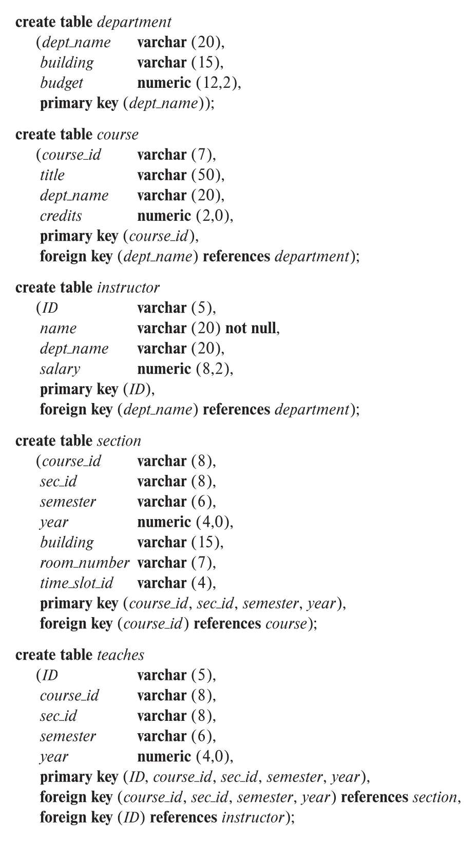Figure 3.1 · PDF p. 99 · university database 일부에 대한 SQL data definition

SQL은 integrity constraint를 위반하는 update를 막는다. Primary key attribute에 null이 들어가거나, 기존 tuple과 primary key 값이 같은 tuple을 insert/update하면 error가 나고 update가 수행되지 않는다. course.dept_name이 department.dept_name에 없는 값을 참조해도 foreign-key constraint 위반으로 insert가 거부된다.

새로 생성된 relation은 initially empty다. Tuple 삽입, 수정, 삭제는 DML statement인 insert, update, delete로 수행하며, 이 장의 3.9절에서 다룬다.

drop table과 delete from은 효과가 다르다.

drop table r;

drop table r은 relation r의 tuple뿐 아니라 schema 정보까지 database에서 제거한다. 이후 r에 tuple을 insert하려면 다시 create table로 relation을 만들어야 한다.

delete from r;

delete from r은 relation schema는 유지하고 모든 tuple만 삭제한다. 즉 빈 table은 남는다.

기존 relation의 schema를 바꾸려면 alter table을 사용한다. Attribute 추가는 다음과 같다.

alter table r add A D;

기존 tuple들은 새 attribute A에 대해 null value를 받는다. Attribute 삭제는 다음처럼 표현한다.

alter table r drop A;

다만 많은 database system은 전체 table drop은 지원해도 attribute drop은 제한적으로 지원하거나 지원하지 않을 수 있다. 이 점은 SQL 표준과 구현체 차이가 드러나는 대표적인 부분이다.

3.3 Basic Structure of SQL Queries

SQL query의 기본 구조는 select, from, where 세 clause로 이루어진다. Query는 from clause에 나열된 relation을 input으로 받고, where와 select가 지정한 방식으로 처리한 뒤, result relation을 만든다.

select A1, A2, ..., An
from r1, r2, ..., rm
where P;

작성 순서는 select → from → where지만, 의미를 이해할 때는 보통 from → where → select 순서로 생각하는 것이 쉽다. from이 대상 relation과 조합을 만들고, where가 tuple predicate로 걸러내며, select가 결과에 남길 attribute 또는 expression을 정한다. 실제 DBMS는 이 순서를 그대로 실행하지 않고 Chapter 15-16에서 다루는 query optimization을 통해 더 효율적인 evaluation plan을 만든다.

3.3.1 Queries on a Single Relation

단일 relation query의 가장 단순한 예는 instructor name 조회다.

select name
from instructor;

from instructor는 input relation을 지정하고, select name은 결과 relation에 name attribute만 남긴다. Relational algebra의 projection과 대응된다.

SQL은 formal relational model과 다르게 duplicate tuple을 기본적으로 허용한다. 예를 들어 모든 instructor의 department name을 조회하면, 같은 department에 여러 instructor가 있으므로 department name이 여러 번 나타난다.

select dept_name
from instructor;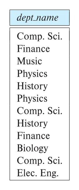

Figure 3.3 · PDF p. 102 · select dept_name from instructor 결과에서 duplicate가 남는 모습

Duplicate를 제거하려면 select distinct를 사용한다.

select distinct dept_name
from instructor;

반대로 duplicate를 제거하지 않겠다는 뜻을 명시하려면 select all을 쓸 수 있지만, duplicate retention이 default이므로 보통은 생략한다. 이 차이는 Chapter 2의 relational algebra가 set semantics를 따르는 것과 SQL이 실용상 bag/multiset semantics를 기본으로 쓰는 차이다. Duplicate elimination은 비용이 들기 때문에 SQL은 기본적으로 제거하지 않는다.

select clause에는 attribute뿐 아니라 arithmetic expression도 올 수 있다.

select ID, name, dept_name, salary * 1.1
from instructor;

이 query는 salary가 10% 인상되었을 때의 값을 결과 relation에 보여줄 뿐, instructor relation을 실제로 바꾸지는 않는다. 실제 modification은 update statement가 담당한다. SQL은 date type 같은 special type과 관련 arithmetic function도 제공하지만, 자세한 type system은 Chapter 4에서 다룬다.

where clause는 from이 만든 tuple 중 predicate를 만족하는 row만 남긴다.

select name
from instructor
where dept_name = 'Comp. Sci.' and salary > 70000;

where predicate에는 and, or, not logical connective와 <, <=, >, >=, =, <> comparison operator를 사용할 수 있다. String, arithmetic expression, date type 등도 비교할 수 있다.

3.3.2 Queries on Multiple Relations

여러 relation이 필요한 query에서는 from에 접근할 relation들을 나열하고, where에 matching condition을 둔다. 예를 들어 instructor name, department name, department building을 함께 보려면 instructor와 department를 dept_name으로 matching해야 한다.

select name, instructor.dept_name, building
from instructor, department
where instructor.dept_name = department.dept_name;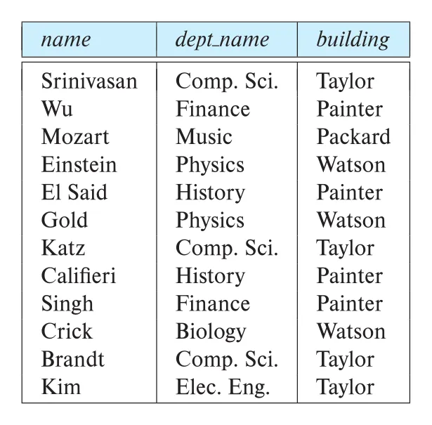

Figure 3.5 · PDF p. 104 · instructor와 department를 dept_name으로 연결한 query 결과

dept_name은 두 relation에 모두 있으므로 instructor.dept_name, department.dept_name처럼 relation-name prefix로 ambiguity를 제거한다. 반면 name과 building은 각각 한 relation에만 있으므로 prefix가 없어도 된다.

SQL query의 각 clause 역할은 다음처럼 요약된다.

Clause	역할	Relational algebra 관점
`select`	결과에 남길 attribute 또는 expression 나열	projection
`from`	접근할 relation 목록	Cartesian product
`where`	tuple을 걸러내는 predicate	selection

from clause에 여러 relation이 있으면 논리적으로 Cartesian product가 만들어진다. 예를 들어 instructor, teaches는 instructor tuple 하나와 teaches tuple 하나를 모두 조합한다. 결과 schema에는 양쪽 relation의 모든 attribute가 들어가며, 같은 attribute name은 instructor.ID, teaches.ID처럼 prefix로 구분한다.

Cartesian product 자체는 대부분 의미 없는 조합을 많이 만든다. 따라서 where clause로 meaningful match만 남겨야 한다.

select name, course_id
from instructor, teaches
where instructor.ID = teaches.ID;

이 query는 instructor와 teaches를 같은 ID 값으로 matching해, 실제로 course를 가르친 instructor의 name과 course id를 출력한다.

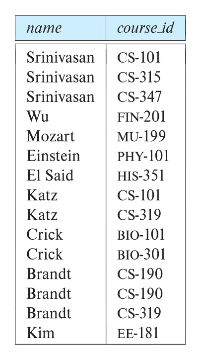Figure 3.7 · PDF p. 107 · instructor.ID = teaches.ID 조건으로 instructor와 teaches를 연결한 결과

Figure 3.7에는 Gold, Califieri, Singh처럼 teaches record가 없는 instructor가 나타나지 않는다. Matching tuple이 없는 쪽도 결과에 남기고 싶다면 Chapter 4의 outer join이 필요하다.

Computer Science department instructor만 보고 싶다면 predicate를 추가한다.

select name, course_id
from instructor, teaches
where instructor.ID = teaches.ID
  and instructor.dept_name = 'Comp. Sci.';

여기서 dept_name은 instructor relation에만 있으므로 instructor.dept_name 대신 dept_name으로 써도 ambiguity는 없다. 다만 여러 relation query에서는 명확성을 위해 prefix를 붙이는 편이 실수를 줄인다.

SQL query의 의미론적 처리 순서는 다음과 같다.

from clause의 relation들로 Cartesian product를 만든다.
where clause의 predicate를 적용해 tuple을 걸러낸다.
남은 tuple마다 select clause의 attribute 또는 expression을 output한다.

이 순서는 결과를 이해하기 위한 conceptual evaluation이다. 실제 DBMS가 정말 거대한 Cartesian product를 먼저 만들면 비효율적이다. 예를 들어 200명 instructor와 600개 teaches tuple이 있으면 naive product는 120,000 tuple을 만든다. 그래서 DBMS는 predicate를 고려해 필요한 조합만 만들도록 query를 최적화한다.

3.4 Additional Basic Operations

3.4.1 The Rename Operation

SQL의 result relation attribute name은 보통 base relation의 attribute name에서 온다. 하지만 두 relation의 attribute 이름이 겹치거나, salary * 1.1처럼 expression을 output하거나, 결과 column 이름을 더 읽기 좋게 바꾸고 싶을 때 rename이 필요하다. SQL은 as clause를 사용한다.

old_name as new_name

예를 들어 result column name을 instructor_name으로 바꿀 수 있다.

select name as instructor_name, course_id
from instructor, teaches
where instructor.ID = teaches.ID;

as는 from clause에서도 relation alias를 만드는 데 사용된다.

select T.name, S.course_id
from instructor as T, teaches as S
where T.ID = S.ID;

Alias는 긴 relation 이름을 줄이는 용도뿐 아니라 같은 relation을 한 query에서 여러 번 참조할 때 필수적이다. 예를 들어 “Biology department의 어떤 instructor보다 salary가 높은 instructor 이름”을 찾으려면 instructor를 두 번 사용해야 한다.

select distinct T.name
from instructor as T, instructor as S
where T.salary > S.salary
  and S.dept_name = 'Biology';

여기서 T와 S는 instructor relation의 물리적 복사본이 아니라 alias다. SQL standard에서는 이런 identifier를 correlation name이라고 부르고, 흔히 table alias, correlation variable, tuple variable이라고도 한다. 같은 relation을 자기 자신과 비교하는 self-join 계열 query에서 alias가 없으면 instructor.salary가 어느 쪽 tuple을 가리키는지 알 수 없다.

Note 3.1은 SQL과 multiset relational algebra의 연결을 설명한다. SQL은 duplicate를 허용하므로, formal relational algebra의 set semantics만으로는 SQL 결과의 tuple copy 수를 설명하기 어렵다. Multiset relational algebra에서는 selection을 통과한 tuple copy 수가 유지되고, projection 후에도 duplicate copy가 남으며, Cartesian product에서는 copy 수가 곱해진다. 기본 SQL query는 개념적으로 다음 multiset relational-algebra expression에 대응한다.

\Pi_{A_1, A_2, \ldots, A_n}(\sigma_P(r_1 \times r_2 \times \ldots \times r_m))

중요한 역사적 용어 함정도 있다. Relational algebra의 select operation은 SQL select clause가 아니라 SQL where clause에 대응한다. SQL select clause는 relational algebra의 projection에 더 가깝다.

3.4.2 String Operations

SQL string은 single quotes로 감싼다. 문자열 안에 single quote 자체를 넣으려면 quote를 두 번 쓴다. 예를 들어 It's right는 SQL string literal로 'It''s right'라고 쓴다.

SQL standard에서 string equality는 case sensitive다. 따라서 'comp. sci.' = 'Comp. Sci.'는 false다. 하지만 MySQL, SQL Server 같은 일부 DBMS는 기본 설정에서 case-insensitive comparison을 할 수 있으므로 구현체 설정을 확인해야 한다.

문자열 함수는 DBMS마다 차이가 있지만, 대표적으로 concatenation(||), substring extraction, length, upper(s), lower(s), trim(s) 등이 있다. Pattern matching은 like operator로 수행하며, 두 special character가 핵심이다.

Pattern 문자	의미
`%`	임의 길이의 substring과 match
`_`	임의의 single character와 match

예시는 다음과 같다.

Pattern	Match 의미
`'Intro%'`	Intro로 시작하는 모든 string
`'%Comp%'`	Comp를 substring으로 포함하는 모든 string
`'___'`	정확히 세 글자인 string
`'___%'`	최소 세 글자인 string

건물 이름에 Watson substring이 포함된 department를 찾는 query는 다음과 같다.

select dept_name
from department
where building like '%Watson%';

%나 _ 자체를 pattern 문자로 해석하지 않고 일반 문자로 찾고 싶다면 escape character를 지정한다.

like 'ab\%cd%' escape '\'

이는 ab%cd로 시작하는 string을 찾는다. Match가 아닌 string을 찾고 싶으면 not like를 쓴다. PostgreSQL 같은 일부 구현체는 Unix regular expression과 비슷한 더 강한 pattern matching인 similar to를 제공한다.

3.4.3 Attribute Specification in the Select Clause

select clause의 *는 “all attributes”를 뜻한다. instructor.*는 result relation에서 instructor relation의 모든 attribute만 선택하고, select *는 from clause 결과 relation의 모든 attribute를 선택한다.

select instructor.*
from instructor, teaches
where instructor.ID = teaches.ID;

*는 탐색이나 임시 확인에는 편하지만, application query에서는 schema 변화에 따라 result column이 조용히 바뀔 수 있으므로 필요한 attribute를 명시하는 편이 안전하다.

3.4.4 Ordering the Display of Tuples

SQL relation 자체에는 tuple order 의미가 없지만, result display 순서는 order by로 지정할 수 있다.

select name
from instructor
where dept_name = 'Physics'
order by name;

기본은 ascending order이며, asc, desc로 방향을 지정할 수 있다. 여러 attribute를 순서 기준으로 줄 수도 있다.

select *
from instructor
order by salary desc, name asc;

이 query는 salary가 높은 순서로 정렬하고, salary가 같은 tuple끼리는 name 오름차순으로 정렬한다.

3.4.5 Where-Clause Predicates

between은 범위 조건을 간결하게 표현한다.

select name
from instructor
where salary between 90000 and 100000;

이는 다음과 같은 의미다.

select name
from instructor
where salary <= 100000 and salary >= 90000;

반대 범위에는 not between을 쓴다. SQL은 row constructor (v1, v2, ..., vn)도 허용한다. Tuple comparison은 lexicographic ordering과 equality를 사용한다. 예를 들어 다음 두 query는 같은 의미로 볼 수 있다.

select name, course_id
from instructor, teaches
where instructor.ID = teaches.ID
  and dept_name = 'Biology';

select name, course_id
from instructor, teaches
where (instructor.ID, dept_name) = (teaches.ID, 'Biology');

다만 row constructor comparison은 SQL-92 표준에 있지만 일부 구현체에서는 지원하지 않을 수 있다.

3.5 Set Operations

SQL의 union, intersect, except는 각각 수학적 set operation인 union(∪), intersection(∩), set difference(-)에 대응한다. 예제로 Fall 2017에 열린 course set c1과 Spring 2018에 열린 course set c2를 사용한다.

select course_id
from section
where semester = 'Fall' and year = 2017;

select course_id
from section
where semester = 'Spring' and year = 2018;

3.5.1 The Union Operation

Fall 2017 또는 Spring 2018에 열린 course를 찾으려면 union을 사용한다.

(select course_id
 from section
 where semester = 'Fall' and year = 2017)
union
(select course_id
 from section
 where semester = 'Spring' and year = 2018);

union은 select와 달리 duplicate를 자동으로 제거한다. Figure 3.10에서 CS-101은 두 semester에 모두 열렸고, CS-319는 Spring 2018에 두 section이 있었지만 결과에는 한 번만 나타난다.

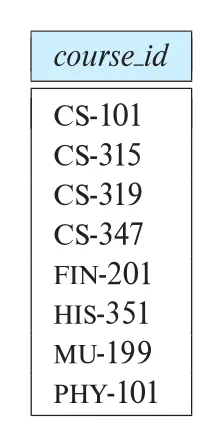Figure 3.10 · PDF p. 116 · c1 union c2 결과에서 duplicate가 제거된 모습

Duplicate를 모두 유지하려면 union all을 사용한다. 이때 result tuple copy 수는 양쪽 input의 copy 수 합이다.

3.5.2 The Intersect Operation

Fall 2017과 Spring 2018에 모두 열린 course를 찾으려면 intersect를 사용한다.

(select course_id
 from section
 where semester = 'Fall' and year = 2017)
intersect
(select course_id
 from section
 where semester = 'Spring' and year = 2018);

intersect도 duplicate를 자동 제거한다. 결과는 양쪽에 모두 등장하는 CS-101이다.

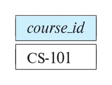Figure 3.11 · PDF p. 116 · c1 intersect c2 결과

intersect all은 duplicate를 유지하며, result copy 수는 양쪽 input copy 수의 minimum이다. 일부 DBMS, 특히 MySQL은 intersect를 직접 지원하지 않아 subquery로 우회해야 할 수 있다.

3.5.3 The Except Operation

Fall 2017에는 열렸지만 Spring 2018에는 열리지 않은 course를 찾으려면 except를 사용한다.

(select course_id
 from section
 where semester = 'Fall' and year = 2017)
except
(select course_id
 from section
 where semester = 'Spring' and year = 2018);

except는 첫 번째 input에 있지만 두 번째 input에는 없는 tuple을 출력하며, set difference처럼 duplicate를 제거하고 계산한다.

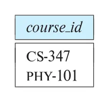Figure 3.12 · PDF p. 117 · c1 except c2 결과

except all은 duplicate를 유지하며, result copy 수는 첫 번째 input copy 수에서 두 번째 input copy 수를 뺀 값이 양수일 때 그 값이다. Oracle은 except 대신 minus를 쓰는 등 구현체 차이가 있고, MySQL은 직접 지원하지 않을 수 있다.

3.6 Null Values

Null value는 SQL operation에서 특별한 문제를 만든다. Arithmetic expression의 input 중 하나가 null이면 결과도 null이다. 예를 들어 r.A + 5에서 r.A가 null이면 결과는 null이다.

Comparison은 더 복잡하다. 1 < null은 true라고 할 수도 없고 false라고 할 수도 없다. Null이 어떤 값을 나타내는지 알 수 없기 때문이다. SQL은 null이 관련된 comparison 결과를 unknown으로 둔다. 따라서 SQL predicate logic에는 true, false, unknown 세 truth value가 있다.

Boolean operation	결과
`true and unknown`	unknown
`false and unknown`	false
`unknown and unknown`	unknown
`true or unknown`	true
`false or unknown`	unknown
`unknown or unknown`	unknown
`not unknown`	unknown

where clause predicate가 false 또는 unknown이면 해당 tuple은 result에 들어가지 않는다. 이 규칙 때문에 null이 있는 column에 대한 비교는 의도보다 tuple을 많이 제거할 수 있다.

Null 여부는 is null, is not null로 검사한다.

select name
from instructor
where salary is null;

SQL은 comparison 결과가 unknown인지 검사하는 is unknown, is not unknown도 정의하지만, 여러 DBMS에서 지원하지 않을 수 있다.

select name
from instructor
where salary > 10000 is unknown;

distinct와 set operation에서 null은 predicate comparison과 다르게 취급된다. Duplicate 제거를 위해 tuple을 비교할 때는 대응 attribute 값이 둘 다 null이면 identical한 것으로 본다. 즉 ('A', null) 두 copy는 select distinct에서 하나만 남는다. 이는 null = null이 predicate에서는 unknown인 것과 구분해야 한다. union, intersect, except에서도 duplicate/identity 판정에는 같은 방식이 쓰인다.

3.7 Aggregate Functions

Aggregate function은 value collection, 즉 set 또는 multiset을 input으로 받아 single value를 반환하는 function이다. SQL의 표준 built-in aggregate function은 다음 다섯 가지다.

Aggregate	의미	입력 제약
`avg`	average	numeric collection
`min`	minimum	numeric뿐 아니라 string 등에도 가능
`max`	maximum	numeric뿐 아니라 string 등에도 가능
`sum`	total	numeric collection
`count`	tuple/value count	tuple 또는 value collection

3.7.1 Basic Aggregation

Computer Science department instructor의 average salary는 다음처럼 구한다.

select avg(salary)
from instructor
where dept_name = 'Comp. Sci.';

Aggregate expression의 result attribute 이름은 DBMS가 어색하게 붙일 수 있으므로 as로 명명하는 것이 좋다.

select avg(salary) as avg_salary
from instructor
where dept_name = 'Comp. Sci.';

Average 계산에서는 duplicate retention이 중요하다. 같은 salary 값을 가진 instructor가 둘 이상 있어도 각각 실제 사람이라면 모두 평균에 들어가야 한다. 반대로 “Spring 2018에 course를 가르친 instructor 수”처럼 instructor가 여러 section을 가르쳐도 한 번만 세야 하는 경우에는 distinct를 aggregate 안에 넣는다.

select count(distinct ID)
from teaches
where semester = 'Spring' and year = 2018;

Tuple 수 자체를 세려면 count(*)를 쓴다.

select count(*)
from course;

SQL은 count(*)에는 distinct를 허용하지 않는다. max와 min에는 distinct를 쓸 수 있지만 결과가 바뀌지 않는다.

3.7.2 Aggregation with Grouping

group by clause는 tuple을 group으로 나눈 뒤 각 group마다 aggregate를 계산한다. 예를 들어 department별 average salary는 다음처럼 쓴다.

select dept_name, avg(salary) as avg_salary
from instructor
group by dept_name;

Figure 3.13은 dept_name 기준으로 instructor tuple들이 group으로 나뉜 모습을 보여준다. 같은 dept_name 값을 가진 tuple들이 한 group이 되고, aggregate function은 group마다 따로 적용된다.

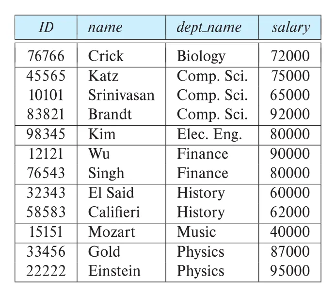Figure 3.13 · PDF p. 122 · dept_name 기준으로 grouped instructor tuples

그 결과는 department별 average salary relation으로 나온다.

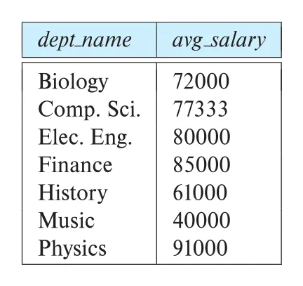Figure 3.14 · PDF p. 122 · department별 avg(salary) query 결과

group by가 없으면 전체 input relation이 하나의 group으로 취급된다. 따라서 select avg(salary) from instructor;는 전체 instructor에 대한 single average를 계산한다.

Join과 grouping을 함께 쓰는 예도 중요하다. Spring 2018에 course를 가르친 instructor 수를 department별로 세려면 teaches에서 semester/year 정보를 얻고, instructor에서 department 정보를 얻어 join한 뒤 group을 만든다.

select dept_name, count(distinct ID) as instr_count
from instructor, teaches
where instructor.ID = teaches.ID
  and semester = 'Spring' and year = 2018
group by dept_name;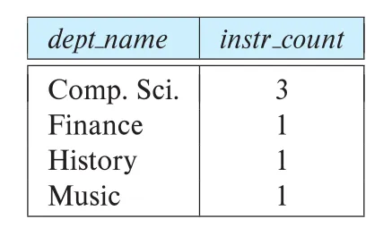

Figure 3.15 · PDF p. 123 · Spring 2018 course를 가르친 instructor 수를 department별로 계산한 결과

Grouping query에서 중요한 규칙은 select clause에 aggregate 없이 나타나는 attribute는 반드시 group by clause에 있어야 한다는 것이다. 다음 query는 erroneous query다.

/* erroneous query */
select dept_name, ID, avg(salary)
from instructor
group by dept_name;

한 department group 안에는 여러 instructor ID가 있을 수 있는데, result tuple은 group당 하나만 나오므로 어떤 ID를 output해야 할지 정의되지 않는다. SQL은 이런 모호한 query를 허용하지 않는다.

SQL comment는 /* ... */로 감싸거나, 한 줄 comment에 --를 사용할 수 있다.

3.7.3 The Having Clause

where는 tuple에 적용되는 predicate이고, having은 group에 적용되는 predicate다. Department별 average salary를 구하되, average salary가 42,000보다 큰 department만 남기려면 다음처럼 쓴다.

select dept_name, avg(salary) as avg_salary
from instructor
group by dept_name
having avg(salary) > 42000;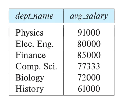

Figure 3.16 · PDF p. 124 · having avg(salary) > 42000을 만족하는 group만 남긴 결과

having에서도 aggregate되지 않은 attribute가 나오려면 group by에 포함되어야 한다. Aggregate query의 의미 순서는 다음과 같다.

from clause를 평가해 relation을 만든다.
where clause가 있으면 tuple-level predicate를 적용한다.
group by가 있으면 남은 tuple을 group으로 나눈다. 없으면 전체가 하나의 group이다.
having clause가 있으면 group-level predicate를 적용해 group을 제거한다.
select clause가 남은 group마다 result tuple을 만든다.

where와 having을 함께 쓰는 예시는 다음과 같다.

select course_id, semester, year, sec_id, avg(tot_cred)
from student, takes
where student.ID = takes.ID and year = 2017
group by course_id, semester, year, sec_id
having count(ID) >= 2;

이 query는 2017년에 열린 각 course section에 대해, 해당 section에 등록한 student의 tot_cred average를 구하되, 등록 student가 2명 이상인 section만 남긴다. Section에 관한 질의처럼 보이지만 필요한 정보가 student와 takes에 모두 있으므로 section relation과 join할 필요는 없다.

3.7.4 Aggregation with Null and Boolean Values

Aggregate function은 null을 특별하게 처리한다. count(*)를 제외한 모든 aggregate function은 input collection에서 null value를 무시한다. 예를 들어 sum(salary)는 salary가 null인 tuple을 제외하고 합계를 계산한다.

select sum(salary)
from instructor;

Null을 무시한 결과 input collection이 empty가 될 수 있다. Empty collection에 대한 count는 0이고, 다른 aggregate operation은 null을 반환한다. SQL:1999에는 true, false, unknown 값을 갖는 Boolean data type이 도입되었고, Boolean collection에 대해 disjunction(or)을 계산하는 some, conjunction(and)을 계산하는 every aggregate가 있다.

Note 3.2는 aggregate가 relational algebra로 어떻게 확장되는지 설명한다. Extended relational algebra의 aggregate operation γ는 grouping attribute와 aggregate expression을 함께 표현한다. 예를 들어 department별 average salary는 개념적으로 다음과 같은 형태다.

{}_{\text{dept\_name}}\gamma_{\operatorname{average}(salary) \to \text{avg\_salary}}(instructor)

SQL의 group by와 having은 relational algebra 관점에서 from/where로 얻은 relation을 group aggregation으로 바꾸고, group-level predicate를 적용한 뒤 projection하는 과정으로 이해할 수 있다.

3.8 Nested Subqueries

Subquery는 다른 query 안에 nested된 select-from-where expression이다. 흔한 용도는 where clause 안에서 set membership을 검사하거나, set comparison을 수행하거나, relation이 empty인지 또는 duplicate가 없는지 검사하는 것이다. 이후 절에서는 where 안의 nested subquery, from 안의 subquery, value expression처럼 쓰이는 scalar subquery를 차례로 다룬다.

3.8.1 Set Membership

in connective는 어떤 tuple 또는 value가 subquery가 만든 relation/set에 속하는지 검사한다. not in은 속하지 않음을 검사한다. Fall 2017에 열렸고 Spring 2018에도 열린 course는 intersect 대신 in으로 쓸 수 있다.

select distinct course_id
from section
where semester = 'Fall' and year = 2017
  and course_id in (select course_id
                    from section
                    where semester = 'Spring' and year = 2018);

여기서 distinct가 필요한 이유는 앞서 intersect가 duplicate를 제거했기 때문이다. 같은 query를 SQL에서 여러 방식으로 쓸 수 있으며, 이는 사용자가 가장 자연스럽게 생각한 방식으로 질의를 표현하게 해 준다.

not in은 set difference와 비슷한 의도를 표현할 수 있다.

select distinct course_id
from section
where semester = 'Fall' and year = 2017
  and course_id not in (select course_id
                        from section
                        where semester = 'Spring' and year = 2018);

in과 not in은 explicit enumerated set에도 쓸 수 있다.

select distinct name
from instructor
where name not in ('Mozart', 'Einstein');

또한 one-attribute relation뿐 아니라 row constructor를 사용해 여러 attribute tuple membership도 검사할 수 있다.

select count(distinct ID)
from takes
where (course_id, sec_id, semester, year) in
      (select course_id, sec_id, semester, year
       from teaches
       where teaches.ID = '10101');

이 query는 특정 instructor가 가르친 section을 들은 distinct student 수를 센다. 다만 (course_id, sec_id, semester, year) 같은 row construction syntax를 모든 SQL implementation이 지원하는 것은 아니다.

3.8.2 Set Comparison

some은 subquery 결과 집합의 원소 중 적어도 하나와 비교 조건을 만족하는지 검사한다. 예를 들어 어떤 Biology department instructor보다 salary가 큰 instructor를 찾으려면 각 instructor salary를 Biology instructor salary 집합과 비교한다.

select name
from instructor
where salary > some (select salary
                     from instructor
                     where dept_name = 'Biology');

> some은 “집합 안의 적어도 하나보다 크다”는 뜻이다. 따라서 Biology instructor salary가 {90000, 100000}이라면 salary 95000은 > some을 만족하지만 > all은 만족하지 않는다. SQL에서는 some 대신 any를 같은 의미로 쓸 수 있다.

비교 연산자와 some의 조합은 직관과 어긋나는 경우가 있다.

표현	의미	주의
`= some`	subquery 결과 중 하나와 같음	`in`과 동일
`<> some`	subquery 결과 중 하나와 다름	`not in`과 다름
`> some`	subquery 결과 중 하나보다 큼	최소값보다 크면 참일 수 있음
`< some`	subquery 결과 중 하나보다 작음	최대값보다 작으면 참일 수 있음

특히 <> some은 “모든 값과 다르다”가 아니다. 예를 들어 {Biology, History}에 대해 dept_name <> some (...)은 대부분의 department에 대해 참이 될 수 있다. Biology도 History와는 다르기 때문이다. “집합에 속하지 않는다”는 조건은 not in 또는 <> all로 표현해야 한다.

all은 subquery 결과 집합의 모든 tuple에 대해 비교 조건이 참인지 검사한다.

select name
from instructor
where salary > all (select salary
                    from instructor
                    where dept_name = 'Biology');

이 query는 Biology department의 모든 instructor보다 salary가 큰 instructor를 찾는다. = all은 “집합의 모든 값과 같다”라는 매우 강한 조건이며, in과 다르다. 반대로 <> all은 subquery의 모든 값과 다르다는 뜻이므로 not in과 동일한 의도로 쓰인다.

all은 최댓값/최솟값을 직접 구하지 않고도 극값 조건을 표현할 수 있다. 예를 들어 department별 average salary 중 가장 높은 department를 찾으려면 각 department의 avg(salary)가 다른 모든 department의 평균 이상인지 검사한다.

select dept_name
from instructor
group by dept_name
having avg(salary) >= all (select avg(salary)
                           from instructor
                           group by dept_name);

동률이 있으면 여러 department가 반환될 수 있다. 이 점은 max()를 사용해 하나의 값만 구한 뒤 비교하는 방식과 같은 의미를 갖지만, SQL에서는 같은 문제를 여러 표현으로 쓸 수 있음을 보여 준다.

3.8.3 Test for Empty Relations

exists는 subquery 결과가 비어 있지 않으면 true를 반환한다. 즉 “조건을 만족하는 tuple이 하나라도 존재하는가?”를 검사한다. 아래 query는 2017년 Fall과 2018년 Spring에 모두 열린 course를 찾는다.

select course_id
from section as S
where semester = 'Fall' and year = 2017
  and exists (select *
              from section as T
              where semester = 'Spring' and year = 2018
                and S.course_id = T.course_id);

안쪽 subquery가 바깥 query의 tuple S.course_id를 참조하므로 이것은 correlated subquery이다. SQL에서는 바깥 query에서 정의된 correlation name이 안쪽 subquery에서 보이며, 더 안쪽 scope에서 같은 이름을 다시 정의하면 local name이 outer name을 가린다.

not exists는 subquery 결과가 empty relation인지 검사한다. 이 패턴은 relational division처럼 “B의 모든 항목을 만족하는 A”를 표현할 때 중요하다. 집합 A가 집합 B를 포함한다는 조건은 B except A가 비어 있다는 말과 같다.

select distinct S.ID, S.name
from student as S
where not exists ((select course_id
                   from course
                   where dept_name = 'Biology')
                  except
                  (select T.course_id
                   from takes as T
                   where S.ID = T.ID));

이 query는 모든 Biology course를 들은 student를 찾는다. 핵심은 “학생이 들은 과목 목록이 Biology course 전체를 포함한다”를 직접 말하지 않고, “Biology course 중 그 학생이 듣지 않은 과목이 존재하지 않는다”로 바꾸는 것이다.

앞 절의 row constructor membership 예시는 exists를 사용해 더 이식성 있게 쓸 수 있다.

select count(distinct ID)
from takes
where exists (select *
              from teaches
              where teaches.ID = '10101'
                and takes.course_id = teaches.course_id
                and takes.sec_id = teaches.sec_id
                and takes.semester = teaches.semester
                and takes.year = teaches.year);

row constructor를 지원하지 않는 implementation에서도 correlated exists는 같은 의미를 표현할 수 있다.

3.8.4 Test for Absence of Duplicate Tuples

unique construct는 subquery 결과에 duplicate tuple이 없으면 true를 반환한다. 예를 들어 2017년에 최대 한 번만 열린 course를 찾을 때 사용할 수 있다.

select T.course_id
from course as T
where unique (select R.course_id
              from section as R
              where T.course_id = R.course_id
                and R.year = 2017);

다만 unique는 널리 구현되어 있지 않다. 같은 의미는 count()로 표현할 수 있다.

select T.course_id
from course as T
where 1 >= (select count(R.course_id)
            from section as R
            where T.course_id = R.course_id
              and R.year = 2017);

not unique는 duplicate가 존재하는지, 즉 같은 tuple이 두 번 이상 나타나는지 검사한다. 그러나 null이 포함된 tuple에서는 주의가 필요하다. SQL에서 null = null은 true가 아니라 unknown이므로, 두 tuple이 값상 비슷해 보여도 equality 비교에서 duplicate로 판정되지 않을 수 있다.

3.8.5 Subqueries in the From Clause

select-from-where expression의 결과는 relation이다. 따라서 SQL은 subquery를 from clause 안에 넣어 derived table처럼 사용할 수 있다.

select dept_name, avg_salary
from (select dept_name, avg(salary) as avg_salary
      from instructor
      group by dept_name)
where avg_salary > 42000;

이 query는 department별 average salary를 먼저 relation으로 만든 뒤, 그 relation에서 평균이 42000보다 큰 row를 고른다. 같은 문제는 having으로도 쓸 수 있지만, from subquery는 중간 결과에 이름을 붙여 복잡한 query를 단계적으로 읽게 해 준다.

Derived table에는 relation 이름과 attribute 이름을 붙일 수 있다.

select dept_name, avg_salary
from (select dept_name, avg(salary)
      from instructor
      group by dept_name)
     as dept_avg(dept_name, avg_salary)
where avg_salary > 42000;

Implementation마다 derived table syntax에는 차이가 있다. MySQL과 PostgreSQL은 from subquery에 이름을 요구하고, Oracle은 derived table 이름 앞의 as를 허용하지 않으며 같은 방식의 attribute rename을 지원하지 않는다. 핵심 개념은 동일하지만, 실제 DBMS에서는 dialect 차이를 확인해야 한다.

from subquery는 여러 단계 aggregate에도 유용하다. 예를 들어 department별 total salary를 만든 뒤 그 total salary의 maximum을 구할 수 있다.

select max(tot_salary)
from (select dept_name, sum(salary) as tot_salary
      from instructor
      group by dept_name);

일반적인 from subquery는 같은 from clause에 앞서 나온 table alias를 참조할 수 없다. SQL:2003의 lateral은 이 제한을 완화한다. lateral subquery는 자기보다 앞에 있는 from item을 참조할 수 있으므로, 각 department에 대해 해당 department instructor들의 평균 salary를 계산하는 식의 correlated derived table을 만들 수 있다.

select name, salary, avg_salary
from instructor I1,
     lateral (select avg(salary) as avg_salary
              from instructor I2
              where I2.dept_name = I1.dept_name);

lateral은 query를 짧게 만들 수 있지만, 모든 DBMS가 같은 문법으로 지원하지는 않는다. PostgreSQL은 lateral을 지원하고, Microsoft SQL Server에서는 비슷한 역할을 cross apply로 표현한다.

3.8.6 With Clause

with clause는 query 안에서만 유효한 temporary relation을 정의한다. 반복되는 subquery에 이름을 붙이거나, 복잡한 query를 논리 단계로 나눌 때 유용하다.

with max_budget(value) as
     (select max(budget)
      from department)
select dept_name
from department, max_budget
where department.budget = max_budget.value;

여기서 max_budget은 실제 table이 아니라 이 query를 처리하는 동안만 존재하는 이름 붙은 relation이다. with는 여러 temporary relation을 함께 정의할 수 있고, 뒤에서 정의된 relation은 앞에서 정의된 relation을 사용할 수 있다.

with dept_total(dept_name, value) as
     (select dept_name, sum(salary)
      from instructor
      group by dept_name),
     dept_total_avg(value) as
     (select avg(value)
      from dept_total)
select dept_name
from dept_total, dept_total_avg
where dept_total.value > dept_total_avg.value;

이 query는 department별 total salary를 계산하고, 그 total의 평균보다 큰 department를 찾는다. 같은 내용을 nested subquery로도 쓸 수 있지만, with는 중간 relation의 의미를 이름으로 드러내므로 읽기 쉽고 유지보수하기 좋다.

3.8.7 Scalar Subqueries

Scalar subquery는 정확히 one tuple, one attribute를 반환하는 subquery이다. SQL은 scalar subquery를 값이 올 수 있는 곳에 둘 수 있다.

select dept_name,
       (select count(*)
        from instructor
        where department.dept_name = instructor.dept_name)
       as num_instructors
from department;

이 query에서 안쪽 subquery는 각 department별 instructor 수라는 단일 값을 만든다. Scalar subquery는 select, where, having clause 등 value expression이 허용되는 곳에 사용할 수 있다. 하지만 실행 시점에 두 개 이상의 tuple이 나오면 runtime error가 발생한다. SQL 표준 관점에서는 subquery 결과가 relation이지만, scalar context에서는 그 relation에서 단일 값을 꺼내 쓰는 셈이다.

3.8.8 Scalar Without a From Clause

일부 DBMS는 from clause 없이 scalar expression만 계산하는 query를 허용한다.

select (select count(*) from teaches) / (select count(*) from instructor);

이 query는 instructor당 평균 teaches tuple 수를 계산하려는 의도이다. 그러나 모든 DBMS가 from 없는 select를 허용하지는 않는다. 그런 system에서는 dummy one-row relation을 사용한다. Oracle은 dual이라는 predefined relation을 제공한다.

또 하나의 실무적 주의점은 numeric division이다. 두 count(*)가 모두 integer이면 결과가 integer division으로 잘릴 수 있다. 정확한 decimal 결과가 필요하면 1.0 *를 곱하거나 적절한 cast를 사용한다.

select (1.0 * (select count(*) from teaches)) /
       (select count(*) from instructor);

Note 3.3 SQL과 Multiset Relational Algebra

SQL의 nested subquery는 기본 relational algebra에 직접 대응되는 단일 연산이 없다. 많은 nested query는 join, projection, selection, aggregation을 조합해 다시 쓸 수 있지만, exists와 not exists를 효율적으로 처리하기 위해 DBMS 내부에서는 semijoin과 antijoin 같은 연산을 사용하기도 한다.

Semijoin은 왼쪽 relation의 tuple 중 오른쪽 relation에 match가 있는 tuple만 남긴다. Antijoin은 반대로 match가 없는 tuple만 남긴다. 이들은 SQL의 표현력을 늘리는 핵심 문법이라기보다, nested query를 실행 계획으로 바꿀 때 유용한 내부 연산으로 이해하면 된다.

3.9 Modification of the Database

SQL은 relation을 조회하는 query language이면서 database content를 바꾸는 DML도 제공한다. 주요 modification은 delete, insert, update이다. 세 연산 모두 relation 전체가 아니라 predicate로 선택된 tuple 집합을 대상으로 작동한다는 점이 중요하다.

3.9.1 Deletion

delete는 relation에서 tuple을 제거한다.

delete from instructor
where dept_name = 'Finance';

where clause를 생략하면 relation의 모든 tuple이 삭제된다.

delete from instructor;

다만 delete from instructor는 relation schema 자체를 없애지 않는다. Table definition을 제거하려면 drop table을 사용해야 한다.

delete는 한 번에 하나의 relation에서만 tuple을 제거한다. 조건을 위해 다른 relation을 subquery로 참조할 수는 있지만, 삭제 대상은 delete from 뒤의 relation 하나이다.

delete from instructor
where dept_name in (select dept_name
                    from department
                    where building = 'Watson');

Aggregate subquery도 삭제 조건에 사용할 수 있다. 예를 들어 전체 평균보다 낮은 salary를 가진 instructor를 삭제할 수 있다.

delete from instructor
where salary < (select avg(salary)
                from instructor);

이때 SQL은 삭제 대상 tuple을 판정할 때 subquery를 각 삭제 이후마다 다시 계산하지 않는다. 먼저 relation의 tuple들을 기준으로 조건을 검사해 삭제할 tuple을 정한 뒤 삭제한다. 그렇지 않으면 평균이 계속 바뀌면서 삭제 결과가 순서에 의존하게 된다.

3.9.2 Insertion

insert는 relation에 새 tuple을 추가한다.

insert into course
values ('CS-437', 'Database Systems', 'Comp. Sci.', 4);

Attribute 순서에 의존하지 않게 하려면 attribute list를 명시한다.

insert into course (course_id, title, dept_name, credits)
values ('CS-437', 'Database Systems', 'Comp. Sci.', 4);

일부 attribute만 명시하면 나머지 attribute에는 null이 들어간다. 단, not null constraint가 있거나 primary key 일부라면 insertion이 거부될 수 있다.

insert는 query 결과 전체를 relation에 추가할 수도 있다.

insert into instructor
select ID, name, dept_name, 18000
from student
where dept_name = 'Music'
  and tot_cred > 144;

중요한 점은 insert ... select에서 select가 먼저 완전히 평가된 뒤 삽입이 일어난다는 것이다. 그렇지 않으면 같은 relation에서 읽고 같은 relation에 쓰는 query가 새로 삽입된 tuple을 다시 읽어 무한히 늘어나는 문제가 생길 수 있다.

대량 data를 넣을 때는 표준 insert 대신 DBMS별 bulk loader utility를 쓰는 경우가 많다. 원리는 같지만, 파일에서 많은 tuple을 효율적으로 적재하도록 최적화되어 있다.

3.9.3 Updates

update는 기존 tuple의 attribute 값을 변경한다.

update instructor
set salary = salary * 1.05;

where clause를 붙이면 조건을 만족하는 tuple만 바꾼다.

update instructor
set salary = salary * 1.05
where salary < 70000;

Nested subquery를 사용해 update 대상을 정할 수도 있다.

update instructor
set salary = salary * 1.05
where salary < (select avg(salary)
                from instructor);

delete와 마찬가지로 update 조건은 기존 relation 상태를 기준으로 판정된다. 각 tuple을 수정할 때마다 average를 다시 계산하는 방식이 아니다.

서로 다른 조건에 서로 다른 update를 적용해야 할 때, 여러 update statement의 순서가 결과에 영향을 줄 수 있다. 예를 들어 salary가 100000 이상이면 3%, 그 미만이면 5% 인상하려고 두 statement를 순서대로 실행하면, 첫 번째 update 이후 salary가 threshold를 넘은 tuple이 두 번째 조건에도 걸리는 문제가 생길 수 있다. 이런 경우 case expression을 사용해 하나의 statement로 처리하는 것이 더 안전하다.

update instructor
set salary = case
               when salary <= 100000 then salary * 1.05
               else salary * 1.03
             end;

case는 조건에 따라 다른 scalar expression을 선택한다. SQL의 case when P then A else B end는 programming language의 if-then-else와 비슷하지만, relation의 각 tuple에 대해 expression으로 평가된다는 점이 중요하다.

update의 set clause에도 scalar subquery를 사용할 수 있다. 예를 들어 student의 tot_cred를 그 학생이 성공적으로 수강한 course credit 합으로 갱신할 수 있다.

update student S
set tot_cred = (select sum(credits)
                from takes, course
                where takes.course_id = course.course_id
                  and S.ID = takes.ID
                  and takes.grade <> 'F'
                  and takes.grade is not null);

하지만 어떤 student가 성공적으로 완료한 course가 하나도 없으면 sum(credits)는 null을 반환한다. tot_cred에 0을 넣고 싶다면 case나 coalesce를 사용해야 한다.

update student S
set tot_cred = (select coalesce(sum(credits), 0)
                from takes, course
                where takes.course_id = course.course_id
                  and S.ID = takes.ID
                  and takes.grade <> 'F'
                  and takes.grade is not null);

coalesce(x, 0)은 x가 null이면 0을, 아니면 x를 반환한다. Aggregate와 null이 결합되는 update에서는 이런 보정이 빠지기 쉽다.

3.10 Summary

Chapter 3의 SQL은 relational model 위에서 실제 database를 정의하고 질의하고 수정하는 언어이다. DDL은 schema와 constraint를 만들고, DML은 tuple을 조회하거나 변경한다. Basic query는 select, from, where로 시작하지만, 실제 SQL은 duplicate를 허용하는 multiset semantics, null과 unknown, aggregation, nested subquery, scalar subquery, with, modification statement까지 포함한다.

SQL을 이해할 때 중요한 축은 두 가지이다. 첫째, 선언적 query가 논리적으로 어떤 relation을 만들고 걸러 내는지 이해해야 한다. 둘째, SQL의 실제 문법과 DBMS별 dialect가 relational algebra의 이상적인 모델과 다를 수 있음을 기억해야 한다. 특히 duplicate, null, aggregate, nested subquery는 SQL을 처음 배울 때 가장 자주 오해되는 부분이다.

연결 관계

Chapter 2의 relational model은 relation, tuple, attribute, domain, key, schema 같은 개념을 정의했다. Chapter 3의 SQL은 그 개념을 실제 언어로 구현한다. create table은 relation schema를 만들고, primary key와 foreign key는 key constraint와 referential integrity를 선언하며, select-from-where는 relational algebra의 selection, projection, Cartesian product, join을 실용 문법으로 표현한다.

Relational algebra와 SQL의 차이도 계속 이어진다. Relational algebra는 기본적으로 set semantics를 가정하지만 SQL은 duplicate를 허용하는 multiset/bag semantics를 기본으로 한다. 그래서 distinct, all, aggregate의 duplicate 처리, set operation의 duplicate elimination을 따로 이해해야 한다.

Nested subquery는 다음 장들의 query optimization과 연결된다. 사용자는 exists, in, all, some, with, scalar subquery로 논리적으로 편한 표현을 쓰지만, DBMS는 이를 join, semijoin, antijoin, aggregation, temporary result 등으로 바꾸어 실행한다. 따라서 “SQL 문장이 어떤 실행 순서로 반드시 돈다”가 아니라 “논리적으로 어떤 결과 relation을 정의한다”는 관점이 중요하다.

Modification statement는 transaction, concurrency control, recovery와 연결된다. Chapter 3에서는 delete, insert, update의 논리 의미를 다루지만, 실제 system에서는 여러 modification이 atomic하게 처리되는지, constraint violation을 어떻게 막는지, failure 후 어떻게 복구되는지가 뒤 장의 핵심 주제가 된다.

오해하기 쉬운 내용

select clause가 SQL 문장 맨 앞에 있지만, basic query의 개념적 평가는 from에서 candidate tuple 조합을 만들고 where로 거른 뒤 select로 결과 attribute를 만든다고 생각하는 것이 좋다.
SQL은 기본적으로 duplicate를 제거하지 않는다. distinct가 없으면 select 결과는 duplicate tuple을 포함할 수 있고, aggregate도 duplicate를 포함해 계산한다.
null은 0이나 empty string이 아니라 unknown/missing value이다. null = null은 true가 아니며, 일반 비교는 unknown을 만들 수 있다.
where clause는 true인 tuple만 통과시킨다. false뿐 아니라 unknown도 결과에서 제외된다.
count(*)는 tuple 수를 세지만 count(attribute)는 해당 attribute가 null이 아닌 tuple만 센다.
sum, avg, min, max는 null을 무시하지만, 입력 tuple이 없거나 모두 null이면 대부분 null을 반환한다. count는 예외적으로 0을 반환할 수 있다.
= some은 in과 같지만 <> some은 not in과 같지 않다. “모든 값과 다르다”는 <> all 또는 not in이다.
exists는 subquery가 반환하는 attribute 값 자체보다 “결과 tuple이 하나라도 있는가”를 본다. 그래서 보통 select *를 써도 논리적으로 충분하다.
with clause로 만든 이름은 영구 table이 아니다. 해당 query 안에서만 유효한 temporary relation이다.
Scalar subquery는 반드시 one tuple, one attribute를 반환해야 한다. 여러 tuple이 나오면 실행 오류가 난다.
delete from r은 table 정의를 지우지 않는다. 모든 tuple을 삭제할 뿐이며 schema를 제거하려면 drop table r이 필요하다.
insert ... select와 조건부 delete/update는 대상 tuple 판정이 statement 실행 전의 논리 상태를 기준으로 이루어진다고 이해해야 순서 의존 오해를 줄일 수 있다.
DBMS별 SQL dialect 차이가 있다. similar to, row constructor membership, unique, lateral, derived table alias syntax, from 없는 scalar query 등은 system마다 지원 범위가 다르다.

면접 질문

SQL에서 DDL과 DML의 차이는 무엇이며, create table, select, insert, update, delete는 각각 어디에 속하는가?
primary key, foreign key, not null constraint가 각각 막아 주는 데이터 이상은 무엇인가?
select distinct dept_name from instructor와 select dept_name from instructor의 결과가 달라질 수 있는 이유는 무엇인가?
SQL의 select-from-where를 relational algebra의 projection, selection, Cartesian product/join과 연결해 설명해 보라.
SQL이 set이 아니라 multiset/bag semantics를 기본으로 한다는 말은 어떤 결과 차이를 만드는가?
order by는 relational model의 relation 개념과 어떤 점에서 긴장이 있는가?
SQL의 null과 three-valued logic에서 unknown이 왜 필요한가? where에서는 unknown이 어떻게 처리되는가?
count(*), count(attribute), count(distinct attribute)의 차이를 예시로 설명해 보라.
where와 having의 차이는 무엇이며, aggregate condition은 왜 보통 having에 두는가?
Correlated subquery란 무엇이고, non-correlated subquery와 실행/의미 측면에서 어떻게 다른가?
in, exists, not exists로 relational division 형태의 “모든 X를 만족하는 Y”를 어떻게 표현할 수 있는가?
some/any와 all의 차이를 설명하고, <> some이 not in과 같지 않은 이유를 말해 보라.
with clause와 from clause의 derived table은 각각 어떤 상황에서 query를 읽기 쉽게 만드는가?
Scalar subquery가 value expression처럼 쓰이려면 어떤 조건을 만족해야 하는가?
delete, insert, update에서 subquery가 포함될 때 statement가 논리적으로 어떤 순서로 평가된다고 이해해야 하는가?
case와 coalesce가 SQL update에서 유용한 상황을 예로 들어 설명해 보라.