개요
Chapter 5의 핵심은 data와 signal을 분리해서 보는 것이다. data는 analog data일 수도 있고 digital data일 수도 있으며, 전송되는 signal도 analog signal 또는 digital signal일 수 있다. 따라서 실제 통신 시스템에서는 네 가지 조합이 생긴다.
- digital data, digital signals
- digital data, analog signals
- analog data, digital signals
- analog data, analog signals
어떤 조합을 고르는지는 transmission medium, available communication facility, bandwidth, error performance, synchronization requirement, 장비 복잡도에 따라 달라진다. 이 장은 “정보를 어떤 파형으로 바꾸어 전송할 것인가”를 다루며, 이후 modulation, multiplexing, physical layer 설계의 기초가 된다.
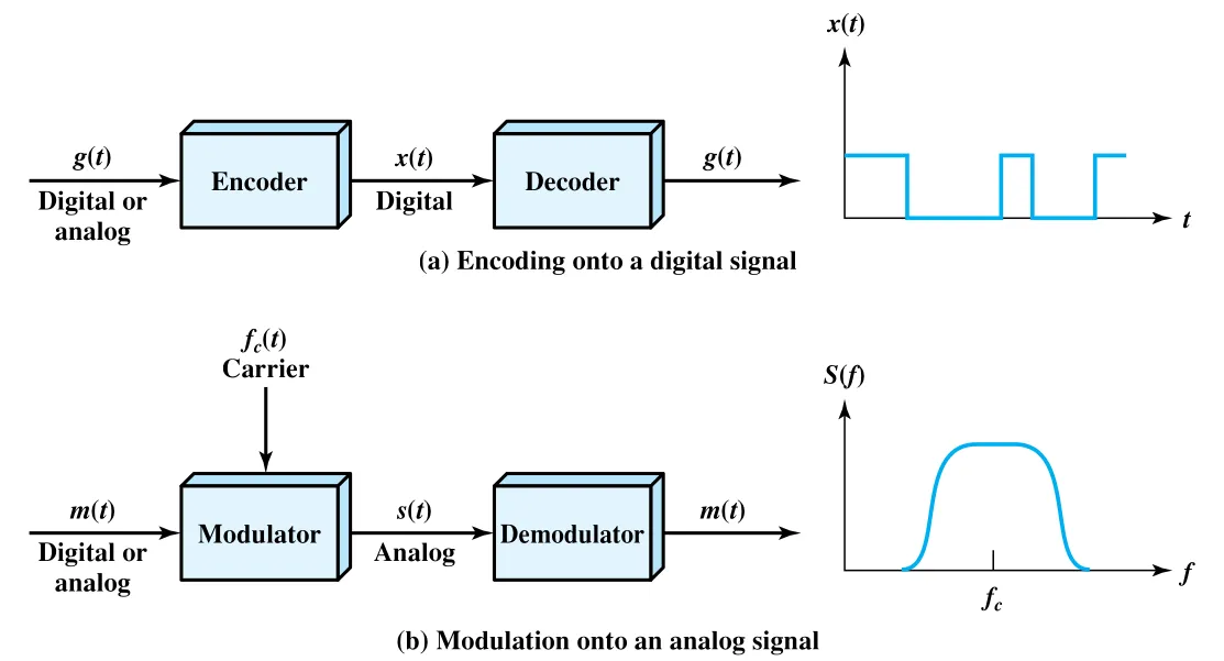 Figure 5.1 · PDF p. 159 · digital signal로의 encoding과 analog carrier로의 modulation 비교
Figure 5.1의 위쪽은 digital signaling이다. source data 는 digital일 수도 analog일 수도 있고, encoder를 거쳐 digital signal 가 된다. 의 실제 모양은 encoding technique에 따라 달라지며, bandwidth를 줄이거나 error를 줄이거나 synchronization을 돕도록 선택된다.
Figure 5.1의 아래쪽은 analog signaling이다. analog signaling의 기반은 carrier signal이다. carrier signal은 일정한 frequency 를 가진 연속 신호이며, data는 modulation을 통해 carrier의 amplitude, frequency, phase 중 하나 이상을 변화시키는 방식으로 실린다. 입력 data 는 modulating signal 또는 baseband signal이라 부르고, modulation 결과는 modulated signal 라 부른다. 는 보통 carrier frequency 주변에 bandwidth가 위치하는 bandpass signal이다.
네 조합을 선택하는 대표 이유는 다음과 같다.
| 조합 | 왜 쓰는가 |
|---|---|
| digital data, digital signal | digital data를 digital signal로 encoding하는 장비가 보통 digital-to-analog modulation 장비보다 단순하고 저렴하다. |
| analog data, digital signal | voice/video 같은 analog data를 digitize하면 modern digital transmission과 digital switching 장비를 사용할 수 있다. |
| digital data, analog signal | optical fiber나 unguided media처럼 특정 매체가 analog signal 형태의 전파를 요구하는 경우가 있다. |
| analog data, analog signal | voice-grade line처럼 analog baseband signal을 싸고 쉽게 전달하거나, bandwidth를 다른 spectrum 위치로 옮겨 FDM(Frequency Division Multiplexing)을 하기 위해 modulation을 쓴다. |
이 장에서 encoding은 넓은 의미로 “data를 transmission에 적합한 signal로 표현하는 방식”이고, modulation은 특히 carrier signal의 성질을 바꾸어 analog signal을 만드는 방식이다.
5.1 Digital Data, Digital Signals
Digital signal은 discrete하고 discontinuous한 voltage pulse들의 sequence다. 각 pulse는 signal element이고, binary data는 data bit를 signal element로 mapping해서 전송된다. 가장 단순한 방식은 bit 하나와 signal element 하나가 1:1로 대응하는 것이다. 그러나 실제 시스템은 bandwidth, synchronization, error performance, cost를 개선하기 위해 더 복잡한 encoding scheme을 쓴다.
기본 용어는 다음처럼 구분해야 한다.
| 용어 | 단위 | 의미 |
|---|---|---|
| data element | bit | binary 1 또는 0 하나 |
| data rate | bps | data element가 전송되는 속도 |
| signal element | digital에서는 voltage pulse | signaling code에서 가장 짧은 구간을 차지하는 신호 단위 |
| signaling rate / modulation rate | baud | signal element가 전송되는 속도 |
| mark / space | - | 역사적 용어로 mark는 1, space는 0 |
receiver가 digital signal을 해석하려면 두 가지를 알아야 한다. 첫째, 각 bit interval이 언제 시작하고 끝나는지 알아야 한다. 둘째, 해당 interval의 signal level이 어떤 binary value를 의미하는지 판단해야 한다. noise, distortion, clock drift가 있으면 sampling 시점이나 threshold 판정이 틀어져 BER(Bit Error Rate)가 증가한다.
encoding scheme을 평가할 때는 다음 기준을 함께 본다.
- Signal spectrum: high-frequency component가 적으면 필요한 bandwidth가 줄고, dc component가 없으면 transformer를 통한 ac coupling과 electrical isolation이 쉬워진다.
- Clocking: 별도 clock lead 없이 transmitted signal 자체에서 synchronization 정보를 얻을 수 있으면 유리하다.
- Error detection: physical signaling 수준에서 일부 오류를 빨리 감지할 수 있으면 좋다.
- Signal interference and noise immunity: 같은 SNR에서 BER이 낮은 code가 유리하다.
- Cost and complexity: 같은 data rate를 위해 더 높은 signaling rate가 필요하면 장비 비용이 증가한다.
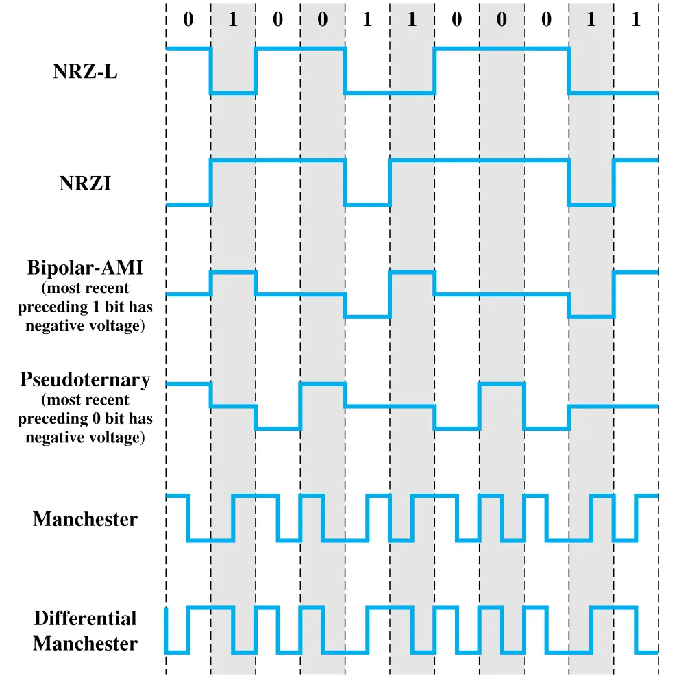 Figure 5.2 · PDF p. 162 · NRZ, multilevel binary, biphase 계열 digital signal encoding waveform
Nonreturn to Zero (NRZ)
NRZ(Nonreturn to Zero)는 bit interval 동안 voltage level이 일정하게 유지되고 zero level로 돌아가지 않는 방식이다. 가장 쉬운 형태는 binary 0과 1에 서로 다른 voltage level을 배정하는 것이다.
NRZ-L(Nonreturn to Zero-Level)은 level 자체가 bit value를 의미한다. 원문 기준에서는 0이 high level, 1이 low level이다. 이 정의는 다른 교재와 반대일 수 있지만, data communications interface와 관련 standards의 관례에 맞춘 것이다. NRZ-L은 terminal이나 device가 digital data를 생성/해석할 때 흔히 쓰이는 기본형이며, 다른 transmission code를 쓸 때도 NRZ-L이 입력 역할을 할 수 있다.
NRZI(Nonreturn to Zero Inverted)는 bit value를 level 자체가 아니라 transition 유무로 표현한다. bit time의 시작에서 transition이 있으면 1, transition이 없으면 0이다. NRZI는 differential encoding의 예다. differential encoding은 현재 signal element의 절대값이 아니라 이전 signal element와의 변화(change)를 정보로 쓴다. 이 방식은 noise 환경에서 threshold level 자체를 판정하는 것보다 transition을 검출하는 편이 더 신뢰할 수 있고, twisted-pair lead가 뒤바뀌어 polarity가 반전되는 상황에도 강하다.
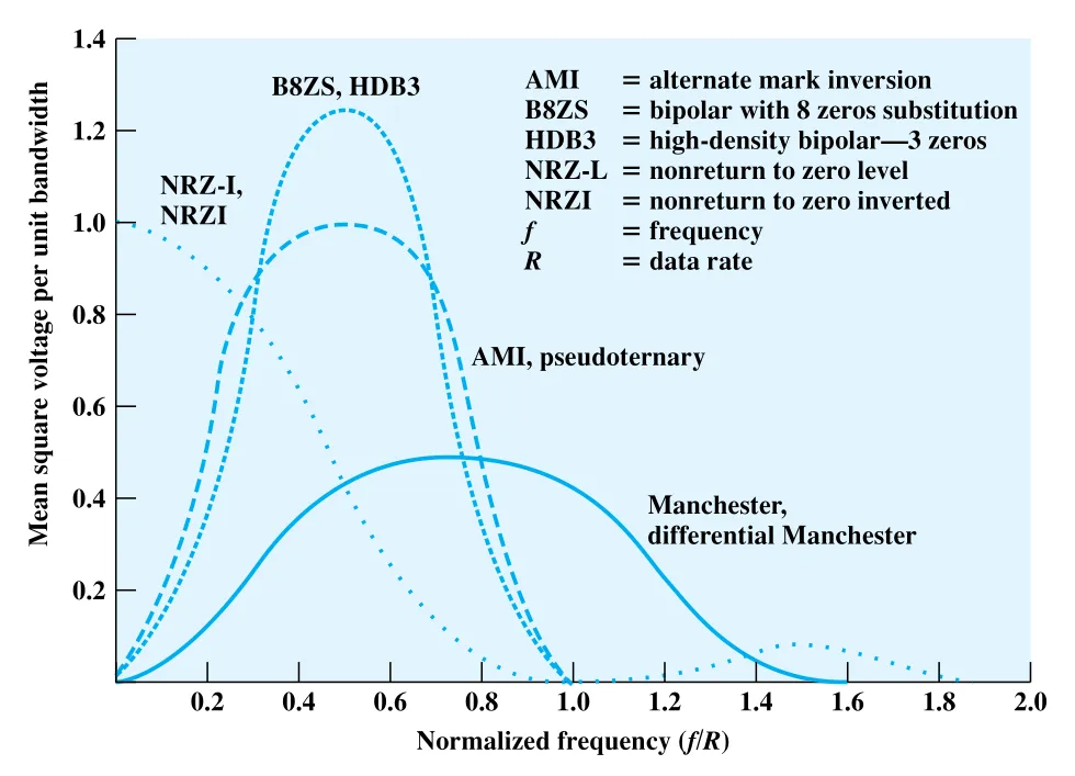 Figure 5.3 · PDF p. 164 · 여러 digital encoding scheme의 spectral density 비교
NRZ의 장점은 engineering이 쉽고 bandwidth를 효율적으로 쓴다는 점이다. Figure 5.3에서 NRZ/NRZI energy는 대체로 dc부터 bit rate의 절반 부근에 집중된다. 예를 들어 9600 bps NRZ signal은 energy 대부분이 dc-4800 Hz 사이에 있다. 그러나 NRZ에는 두 가지 큰 약점이 있다. 첫째, dc component가 있다. 둘째, 긴 0 또는 긴 1 sequence에서 transition이 없어 synchronization을 잃기 쉽다. 그래서 NRZ는 digital magnetic recording에는 유용하지만 signal transmission application에는 한계가 있다.
Multilevel Binary
Multilevel binary는 두 개보다 많은 signal level을 사용하는 encoding 계열이다. 대표 예는 Bipolar-AMI(Alternate Mark Inversion)와 pseudoternary다.
Bipolar-AMI에서는 binary 0을 no line signal로 표현하고, binary 1을 positive 또는 negative pulse로 표현하되 successive ones의 polarity를 번갈아 바꾼다. 이 방식의 장점은 세 가지다. 긴 1 sequence에서는 매 bit마다 transition이 생겨 synchronization에 도움이 된다. positive pulse와 negative pulse가 번갈아 나오므로 net dc component가 없다. 또한 같은 polarity가 연속되는 식의 AMI rule violation은 error detection 단서가 된다.
Pseudoternary는 반대로 binary 1을 no line signal로, binary 0을 alternating positive/negative pulse로 표현한다. 원리는 AMI와 비슷하며 어느 쪽이 절대적으로 우월하다기보다 application별 관례가 다르다.
하지만 AMI는 긴 0 sequence에서, pseudoternary는 긴 1 sequence에서 transition이 없어 synchronization 문제가 남는다. 또한 multilevel binary는 receiver가 세 level을 구분해야 하므로 two-level signal보다 noise margin이 작다. 원문은 같은 bit error probability를 얻기 위해 multilevel binary가 two-valued signal보다 약 3 dB 더 많은 signal power를 요구한다고 설명한다.
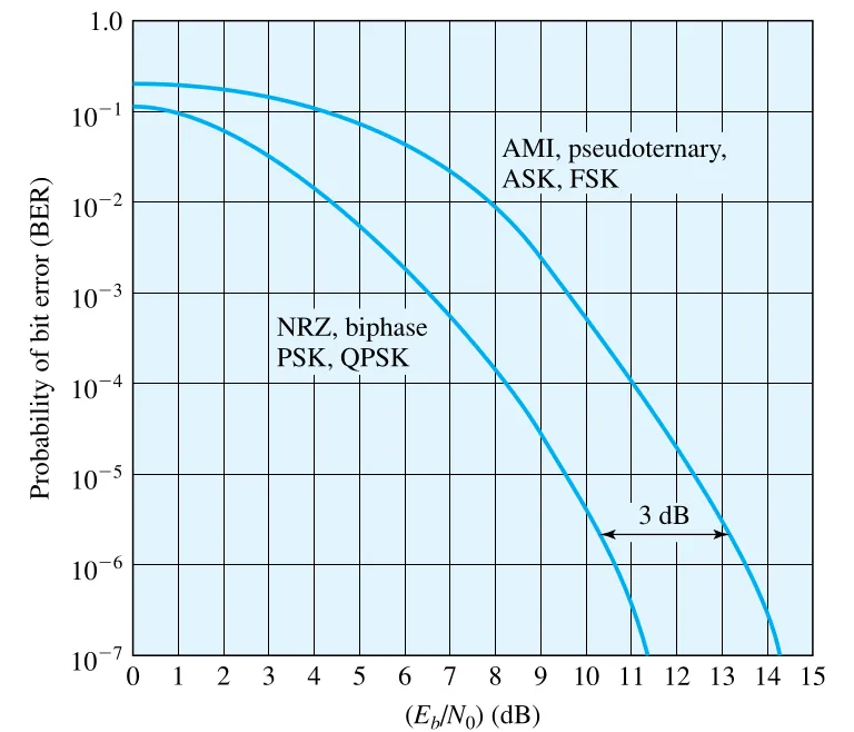 Figure 5.4 · PDF p. 166 · NRZ/biphase와 AMI/pseudoternary의 theoretical BER 비교
Figure 5.4는 같은 조건에서 NRZ/biphase 계열과 AMI/pseudoternary 계열의 BER 차이를 보여준다. line code 선택은 단순히 waveform이 예쁜지를 고르는 문제가 아니라, bandwidth, synchronization, dc component, required power, BER 사이의 trade-off다.
Biphase
Biphase 계열의 대표 방식은 Manchester와 Differential Manchester다. Manchester code는 bit period의 한가운데에 항상 transition을 둔다. 이 midbit transition은 clocking mechanism이면서 동시에 data를 표현한다. 원문 기준에서 low-to-high transition은 1, high-to-low transition은 0이다. 이 정의 역시 일부 교재와 반대일 수 있지만, IEEE 802.3 Ethernet 등 industry practice를 따른다.
Differential Manchester는 midbit transition을 clocking 전용으로 사용한다. bit period 시작에서 transition이 있으면 0, 없으면 1이다. 따라서 differential encoding의 장점도 함께 가진다.
Biphase의 장점은 분명하다. 매 bit time마다 예측 가능한 transition이 있으므로 self-clocking code가 된다. dc component가 없다. 기대한 transition이 없으면 error detection에도 사용할 수 있다. 단점은 signal transition이 많아 maximum modulation rate가 NRZ보다 커지고, 그만큼 bandwidth requirement가 증가한다는 점이다. Figure 5.3에서 biphase의 bandwidth는 multilevel binary보다 넓다.
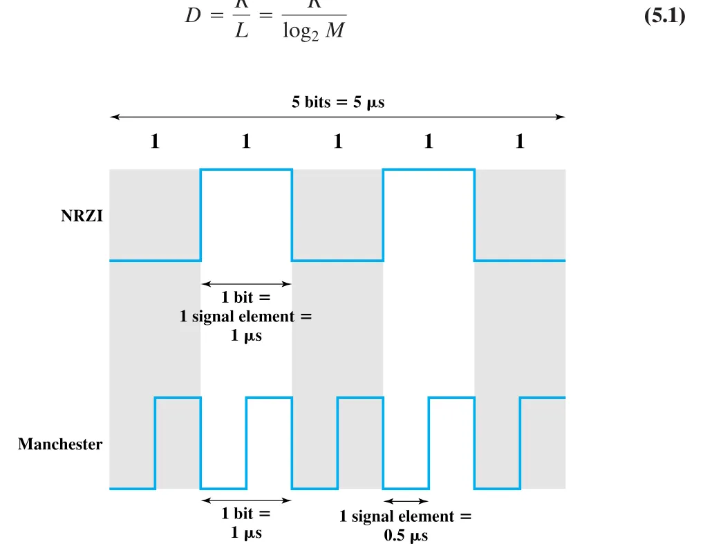 Figure 5.5 · PDF p. 167 · 1 Mbps binary ones stream에서 NRZI와 Manchester의 signaling rate 차이
data rate와 modulation rate는 반드시 구분해야 한다. data rate는 bit per second이고, modulation rate는 signal elements per second, 즉 baud다. Manchester encoding에서는 bit interval 절반짜리 pulse가 최소 signal element가 될 수 있으므로, all 0s 또는 all 1s에서는 maximum modulation rate가 까지 올라간다.
여기서 는 modulation rate, 은 data rate, 은 서로 다른 signal element 수, 은 signal element당 bit 수다. 같은 bps라도 encoding 방식에 따라 필요한 baud와 bandwidth가 달라진다는 점이 이 절의 핵심이다.
Scrambling Techniques
Biphase는 LAN의 비교적 높은 data rate에서는 널리 쓰였지만, long-distance application에서는 signaling rate가 data rate에 비해 높아 비효율적이다. 이를 피하기 위한 접근이 scrambling이다. scrambling은 line에 constant voltage level을 만들 sequence를 transition이 충분한 filling sequence로 바꾸고, receiver가 그 pattern을 다시 원래 data sequence로 복원하게 한다. filling sequence는 원래 sequence와 같은 길이이므로 data rate penalty가 없다.
scrambling scheme의 목표는 no dc component, long zero-level line signal 방지, no reduction in data rate, error-detection capability다. 대표 방식은 B8ZS와 HDB3다.
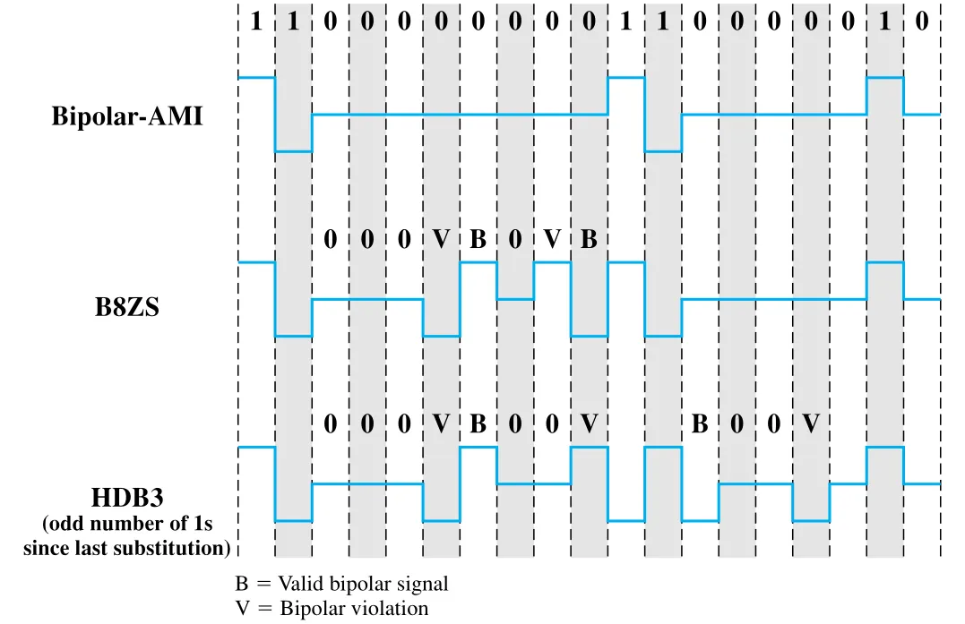 Figure 5.6 · PDF p. 169 · B8ZS와 HDB3가 긴 zero sequence를 bipolar violation pattern으로 대체하는 규칙
B8ZS(Bipolar with 8-Zeros Substitution)는 AMI 기반이며, all-zero octet이 나오면 AMI에서는 불가능한 두 개의 code violation을 포함하는 pattern으로 바꾼다. noise가 우연히 이런 violation pattern을 만들 가능성은 낮으므로 receiver는 이를 인식해 원래의 eight zeros로 복원한다.
HDB3(High-Density Bipolar-3 zeros)는 AMI 기반으로 네 개의 zero string을 one or two pulse를 포함한 sequence로 대체한다. 네 번째 zero는 code violation으로 바뀌며, successive violations가 alternate polarity가 되도록 preceding pulse polarity와 마지막 substitution 이후 pulse 수의 odd/even 여부를 사용한다. 이렇게 하면 dc component를 만들지 않으면서 transition을 확보할 수 있다.
B8ZS와 HDB3는 대부분의 energy가 data rate의 절반 부근에 비교적 sharp하게 집중되고 dc component가 없어서 high data rate transmission에 적합하다.
5.2 Digital Data, Analog Signals
Digital data를 analog signal로 보내는 대표 상황은 public telephone network를 통한 data 전송이다. 전통적 telephone network는 subscriber location에서 들어오는 digital signal을 직접 처리하도록 설계된 것이 아니라, 약 300-3400 Hz voice-frequency range의 analog signal을 receive, switch, transmit하도록 설계되었다. 그래서 digital device는 modem(modulator-demodulator)을 통해 digital data를 analog signal로 바꾸고, 반대 방향에서는 analog signal을 다시 digital data로 복원한다.
digital data를 analog signal로 변환하는 기본 방식은 carrier signal의 amplitude, frequency, phase를 바꾸는 것이다. 각각 ASK(Amplitude Shift Keying), FSK(Frequency Shift Keying), PSK(Phase Shift Keying)라고 부른다. 세 방식 모두 결과 signal은 carrier frequency 주변에 centered bandwidth를 가진다.
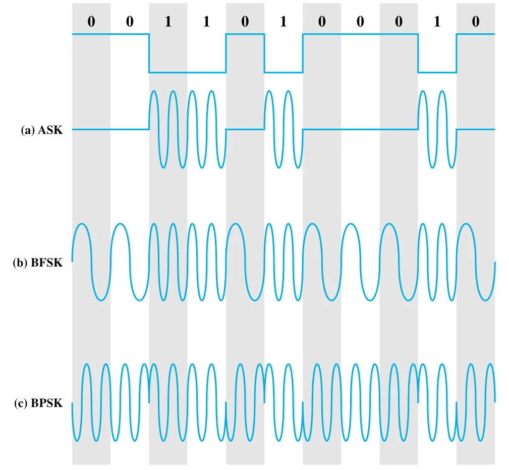 Figure 5.7 · PDF p. 171 · digital data를 analog carrier에 싣는 ASK, BFSK, BPSK waveform
Amplitude Shift Keying (ASK)
ASK에서는 두 binary value를 carrier의 서로 다른 amplitude로 표현한다. 흔한 형태는 carrier가 존재하면 1, carrier가 없으면 0으로 보는 것이다.
ASK는 sudden gain change에 취약하고 modulation 효율도 좋지 않다. voice-grade line에서는 보통 1200 bps 이하 정도에 쓰인다. 다만 optical fiber에서는 digital data를 빛의 pulse 유무 또는 lightwave amplitude 차이로 표현하는 방식이 ASK와 같은 구조를 가진다. LED transmitter에서는 light pulse와 no light가 signal element를 구분하고, laser transmitter에서는 낮은 bias light level과 더 높은 light level이 서로 다른 signal element를 나타낼 수 있다.
Frequency Shift Keying (FSK)
FSK에서는 binary value를 서로 다른 frequency로 표현한다. 가장 흔한 형태는 BFSK(Binary FSK)로, carrier frequency 근처의 두 frequency 가 1과 0을 나타낸다.
보통 과 는 를 중심으로 같은 크기만큼 반대 방향으로 offset된다. BFSK는 ASK보다 error에 덜 취약하며, voice-grade line에서는 보통 1200 bps 이하, high-frequency radio transmission이나 coaxial cable 기반 LAN에서도 쓰일 수 있다.
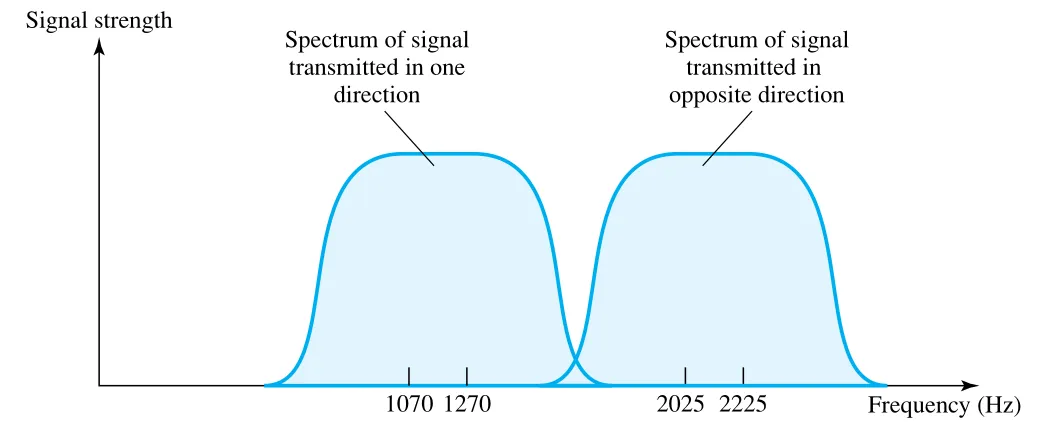 Figure 5.8 · PDF p. 172 · voice-grade line에서 BFSK full-duplex를 위해 frequency band를 나누는 예
Figure 5.8은 voice-grade line의 300-3400 Hz bandwidth 안에서 full-duplex BFSK를 구성하는 방식이다. 한 방향은 1170 Hz 중심에 ±100 Hz shift를 두고, 반대 방향은 2125 Hz 중심에 ±100 Hz shift를 둔다. 두 방향의 spectrum overlap을 작게 만들어 동시에 양방향 전송해도 interference가 작도록 한다.
Multiple FSK (MFSK)
MFSK(Multiple FSK)는 두 개보다 많은 frequency를 사용한다. 각 signaling element가 bits를 표현하므로 개의 서로 다른 frequency가 필요하다.
각 output signal element는 동안 유지된다. 여기서 는 input bit period다. 한 signal element가 bits를 묶어 표현하므로 symbol duration은 길어지지만, 필요한 frequency tone 수와 bandwidth는 증가한다. 원문은 total bandwidth를 , minimum frequency separation 조건을 , 따라서 로 설명한다.
MFSK는 bandwidth efficiency 측면에서는 불리할 수 있지만, frequency 간 구분을 이용해 robustness를 얻는 방향의 설계다. 즉 더 많은 frequency slot을 쓰는 대신 하나의 symbol이 여러 bit를 담고, tone 구분으로 data를 표현한다.
Phase Shift Keying (PSK) 기본형
PSK에서는 carrier의 phase를 바꾸어 data를 표현한다. 가장 단순한 방식은 BPSK(Binary PSK)로, 두 phase가 binary 1과 0을 나타낸다. 180도 phase shift는 sine wave를 뒤집는 것과 같으므로 다음처럼 표현할 수 있다.
BPSK는 ASK/FSK보다 같은 조건에서 error performance가 좋은 축에 속하며, 이후 QPSK, MPSK, QAM으로 확장된다.
Differential PSK (DPSK)
BPSK는 bit value를 fixed reference phase와 비교해 표현한다. 이를 편리하게 쓰면 bit가 1일 때 , 0일 때 인 discrete function으로 두고 다음처럼 표현할 수 있다.
DPSK(Differential PSK)는 phase를 절대 기준이 아니라 이전 symbol에 대한 변화로 표현한다. binary 0은 이전 signal burst와 같은 phase, binary 1은 이전 signal burst와 반대 phase를 보낸다. receiver가 transmitter와 정확히 phase가 일치하는 local oscillator를 유지하지 않아도 되고, 직전 phase가 올바르게 수신되었다면 그것을 기준으로 다음 symbol을 판단할 수 있다.
 Figure 5.10 · PDF p. 174 · 이전 burst와의 phase 변화로 bit를 표현하는 DPSK 예
Four-Level PSK: QPSK와 OQPSK
Bandwidth를 더 효율적으로 쓰려면 signal element 하나가 bit 하나보다 많은 정보를 담아야 한다. QPSK(Quadrature Phase Shift Keying)는 , 즉 간격의 네 phase를 사용해 symbol 하나가 2 bits를 표현하게 한다. 예를 들어 네 bit pair를 각각 서로 다른 phase에 배정한다.
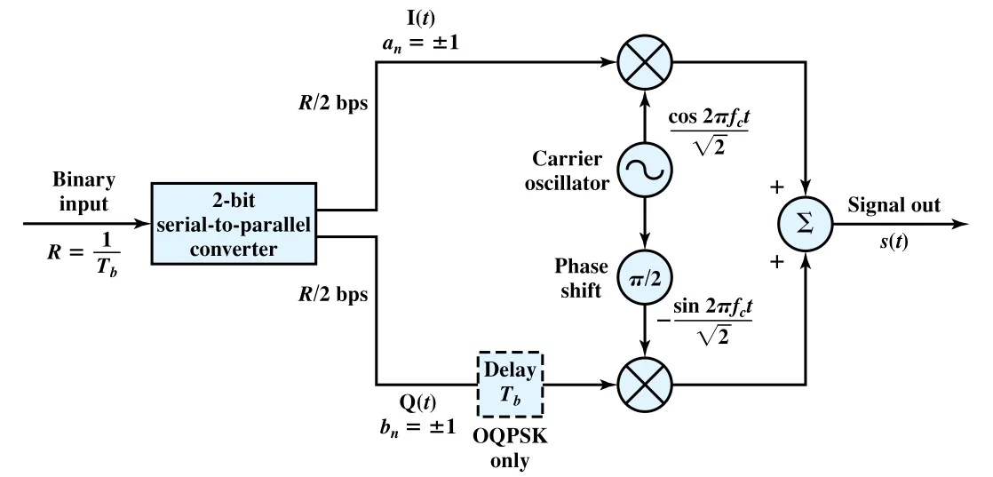 Figure 5.11 · PDF p. 175 · input bit stream을 I/Q 두 stream으로 나누어 QPSK/OQPSK를 만드는 modulator
QPSK modulator는 input bit stream을 alternate bits로 나누어 두 개의 bps stream으로 만든다. 하나는 I(in-phase) stream, 다른 하나는 Q(quadrature phase) stream이다. I stream은 carrier에, Q stream은 90도 shift된 carrier에 실리고 두 결과가 더해져 전송된다.
각 I/Q stream은 원래 bit rate의 절반이므로 combined signal의 symbol rate는 input bit rate의 절반이다. 즉 QPSK는 같은 symbol rate로 BPSK보다 두 배의 data rate를 낼 수 있다.
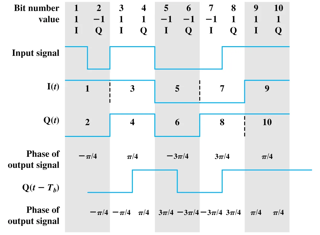 Figure 5.12 · PDF p. 176 · QPSK와 OQPSK waveform에서 phase 변화 폭이 달라지는 모습
OQPSK(Offset QPSK, Orthogonal QPSK)는 Q stream에 one bit time delay를 넣은 QPSK 변형이다. spectral characteristics와 bit error performance는 QPSK와 같지만, 한 symbol time에서 I/Q 중 하나만 sign이 바뀌도록 만들어 combined phase change가 를 넘지 않게 한다. phase modulator가 큰 phase shift를 빠르게 수행하기 어렵거나, transmitter/receiver/channel에 nonlinear component가 있어 bandwidth spreading과 adjacent channel interference가 걱정되는 경우 OQPSK가 유리하다.
Multilevel PSK와 Bandwidth Efficiency
Multilevel PSK(MPSK)는 2 bits뿐 아니라 3 bits 이상을 하나의 signal element에 담도록 phase level 수를 늘린다. 예를 들어 개의 signal element를 쓰면 bits가 symbol 하나에 담긴다. 그러면 data rate가 9600 bps라도 line signaling speed는 2400 baud가 될 수 있다. 이것이 voice-grade line에서 더 높은 bit rate를 얻기 위해 complex modulation을 쓰는 이유다.
Bandwidth efficiency는 , 즉 transmission bandwidth당 data rate다. 원문이 제시한 기본 관계는 다음과 같다.
| 방식 | transmission bandwidth 의 경향 | 증가 효과 |
|---|---|---|
| ASK/PSK | 기본 2-level에서는 bit rate와 직접 비례 | |
| MPSK | 이 커질수록 bandwidth efficiency 증가 | |
| MFSK | 이 커질수록 bandwidth efficiency 감소 |
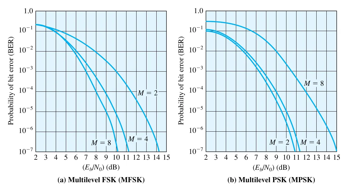 Figure 5.13 · PDF p. 178 · MFSK와 MPSK에서 level 수 M에 따른 BER trade-off
Figure 5.13의 중요한 메시지는 MFSK와 MPSK가 정반대 방향의 trade-off를 가진다는 점이다. MFSK는 이 증가하면 같은 에서 error probability가 낮아지지만 bandwidth efficiency가 나빠진다. MPSK는 이 증가하면 bandwidth efficiency가 좋아지지만 phase 간 간격이 좁아져 error probability가 높아진다. 결국 multilevel signaling은 “더 많은 bit를 symbol 하나에 넣는 대신 noise margin을 줄이는가” 또는 “더 넓은 bandwidth를 쓰고 더 robust하게 가는가”의 선택이다.
Quadrature Amplitude Modulation (QAM)
QAM(Quadrature Amplitude Modulation)은 ASK와 PSK를 결합한 analog signaling technique이다. ADSL과 일부 wireless standards에서 사용된다. QAM은 같은 carrier frequency의 두 copy를 사용하되, 하나를 다른 하나에 대해 90도 phase shift한다. 두 carrier는 서로 orthogonal하므로 같은 frequency 위에서 두 독립 signal을 동시에 보낼 수 있다.
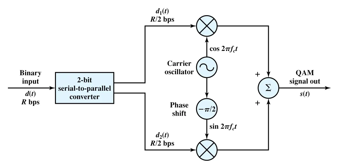 Figure 5.14 · PDF p. 180 · input bit stream을 두 stream으로 나누어 I/Q ASK modulation으로 결합하는 QAM modulator
QAM modulator는 input stream 를 bps의 두 stream 로 나눈다. 는 , 는 carrier에 실리고 두 신호가 더해진다.
두 stream이 각각 two-level ASK라면 combined signal은 states를 가지며 이는 본질적으로 QPSK와 유사하다. four-level ASK를 쓰면 states가 되고, 64-state, 256-state QAM도 가능하다. state 수가 많을수록 같은 bandwidth에서 더 높은 data rate를 낼 수 있지만, noise와 attenuation에 의해 symbol decision error가 증가할 수 있다.
5.3 Analog Data, Digital Signals
Analog data를 digital signal로 바꾸는 과정은 엄밀히 말하면 analog data를 digital data로 변환하는 digitization이다. analog data가 digitize되면 이후에는 세 가지 방식으로 전송될 수 있다. NRZ-L 같은 digital signal로 바로 보낼 수도 있고, 다른 digital line code로 다시 encoding할 수도 있으며, 필요하면 5.2의 modulation technique을 사용해 analog signal로 다시 변환할 수도 있다.
 Figure 5.15 · PDF p. 181 · voice analog data를 digitize한 뒤 ASK analog signal로 다시 변환하는 예
Figure 5.15는 겉보기에는 이상한 경로를 보여준다. analog voice data를 digitize한 뒤 다시 ASK analog signal로 보낸다. 그러나 이는 transmission requirement가 microwave 같은 analog signal 전송을 요구하더라도, voice가 이미 digitized data가 되었기 때문에 digital transmission의 장점을 일부 활용할 수 있음을 보여준다.
analog data를 digital form으로 변환하고, 수신 측에서 다시 analog data로 복원하는 장치를 codec(coder-decoder)이라고 한다. 대표 codec technique은 PCM(Pulse Code Modulation)과 DM(Delta Modulation)이다.
Pulse Code Modulation (PCM)
PCM은 sampling theorem에 기반한다.
signal 를 regular interval로 sample하고, sampling rate가 highest signal frequency의 두 배보다 크면, sample들은 original signal의 모든 정보를 포함한다. 이 sample들로 lowpass filter를 통해 를 재구성할 수 있다.
예를 들어 voice data를 4000 Hz 이하로 제한하면, 8000 samples/second가 voice signal을 표현하기에 충분하다. 이때 얻는 sample은 아직 analog amplitude를 가진 PAM(Pulse Amplitude Modulation) sample이다. digital data로 만들려면 각 sample을 quantizing level 중 하나에 배정하고 binary code를 붙여야 한다.
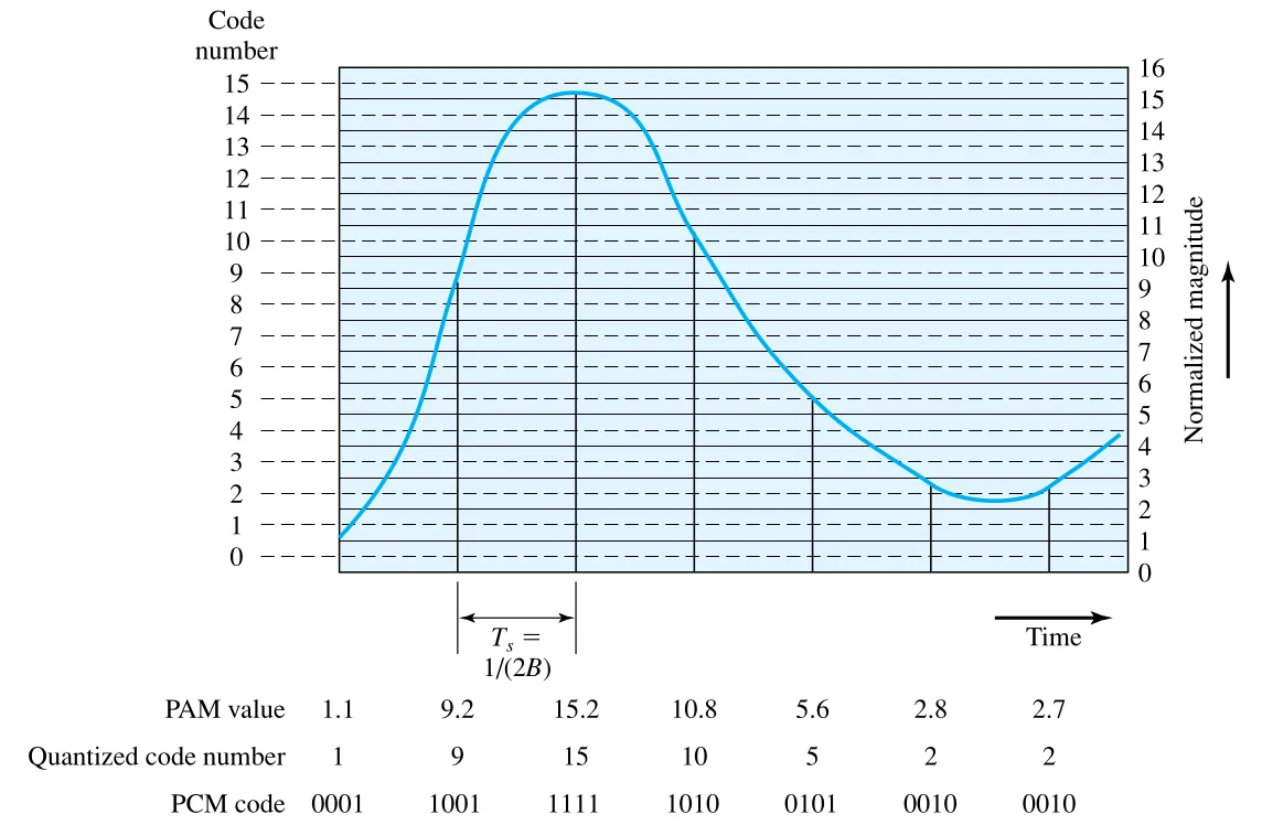 Figure 5.16 · PDF p. 182 · analog waveform을 PAM sample로 잡고 quantized code number와 PCM code로 바꾸는 예
Figure 5.16은 bandwidth 인 analog signal을 rate로 sampling하고, sample amplitude를 16개 quantizing level 중 하나로 근사한 뒤 4-bit PCM code로 표현하는 과정을 보여준다. 일반 voice 품질에서는 8-bit sample, 즉 256 quantizing levels가 널리 쓰이며, 8000 samples/second와 결합하면 single voice signal에 kbps가 필요하다.
 Figure 5.17 · PDF p. 183 · PAM sampler, quantizer, encoder로 이어지는 PCM block diagram
PCM block은 analog input을 PAM sampler로 discrete-time continuous-amplitude signal로 만들고, quantizer로 discrete-amplitude pulse로 만든 뒤, encoder가 digital bit stream을 만든다. 수신 측에서는 이 과정을 반대로 수행해 analog signal을 재구성한다. 하지만 quantizing은 sample amplitude를 근사값으로 바꾸므로 original signal을 정확히 복구할 수 없다. 이 오차를 quantizing error 또는 quantizing noise라고 한다.
quantizing noise에 대한 SNR은 다음처럼 근사된다.
따라서 quantizing bit를 1 bit 늘릴 때마다 SNR은 약 6 dB 증가한다. 6 dB는 power ratio로 약 4배에 해당한다.
Nonlinear Encoding과 Companding
uniform quantization에서는 sample amplitude가 작든 크든 평균 절대 error가 비슷하다. 그러면 low-amplitude signal은 상대적으로 더 크게 왜곡된다. 이를 줄이기 위해 nonlinear encoding은 quantization level을 균등하게 배치하지 않는다. low-amplitude region에는 더 많은 quantizing step을 주고, large-amplitude region에는 더 적은 step을 둔다.
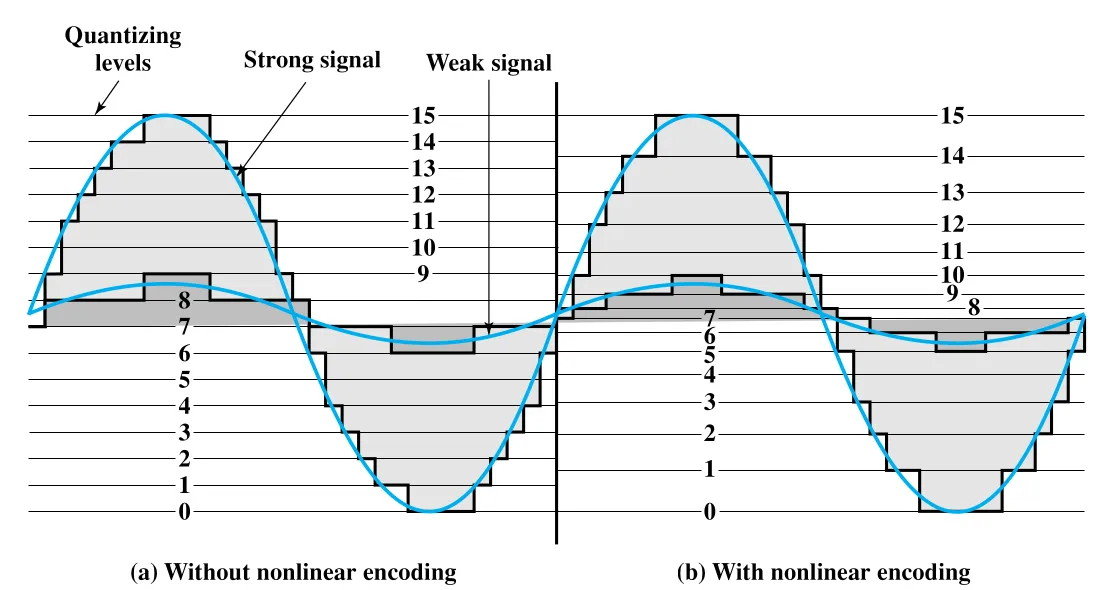 Figure 5.18 · PDF p. 183 · nonlinear coding이 weak signal에 더 촘촘한 quantizing level을 제공하는 효과
같은 효과는 uniform quantizing과 companding(compressing-expanding)을 결합해 얻을 수도 있다. 송신 전 input analog signal의 intensity range를 compress하되 weak signal에 strong signal보다 더 큰 gain을 주고, 수신 후에는 반대로 expand한다.
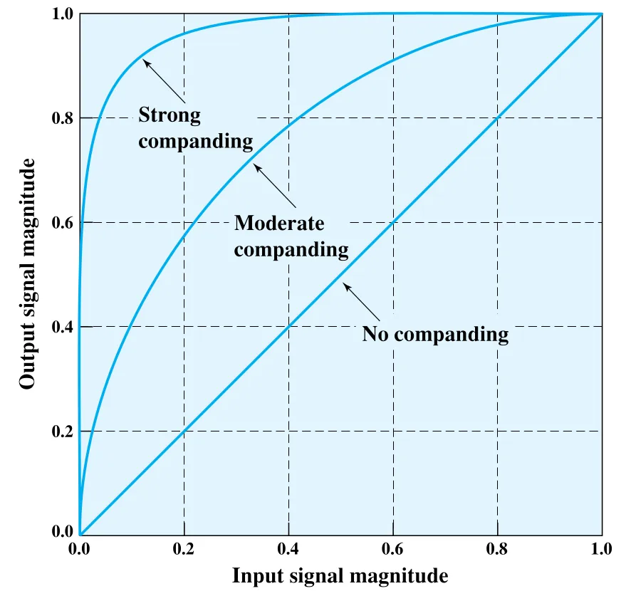 Figure 5.19 · PDF p. 184 · no/moderate/strong companding function의 input-output 관계
Companding의 input side에서는 큰 sample value가 상대적으로 눌리므로, fixed number of quantizing levels 중 더 많은 level이 low-level signal 표현에 쓰인다. output side에서는 compressed value가 원래 range로 확장된다. voice signal에서는 nonlinear encoding과 companding으로 PCM SNR을 24-30 dB 정도 개선할 수 있다.
Delta Modulation (DM)
DM(Delta Modulation)은 PCM보다 단순한 대안이다. analog input을 staircase function으로 근사하고, 각 sampling interval 마다 staircase가 step size 만큼 올라갈지 내려갈지만 결정한다. 즉 sample 하나당 amplitude 값을 여러 bit로 보내는 것이 아니라, “다음 interval에 up인가 down인가”를 1 bit로 보낸다.
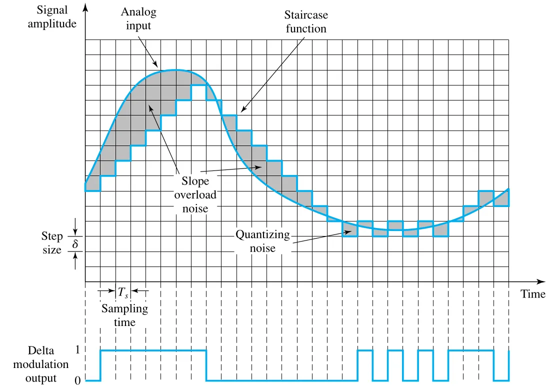 Figure 5.20 · PDF p. 185 · delta modulation의 staircase approximation, quantizing noise, slope overload noise
DM은 analog signal의 amplitude 자체보다 derivative를 근사하는 방식으로 이해하면 좋다. staircase function이 다음 interval에 올라가야 하면 1, 내려가야 하면 0을 생성한다. 수신 측은 이 binary sequence로 동일한 staircase function을 재구성하고, integration 또는 lowpass filter로 smoothing해 analog approximation을 얻는다.
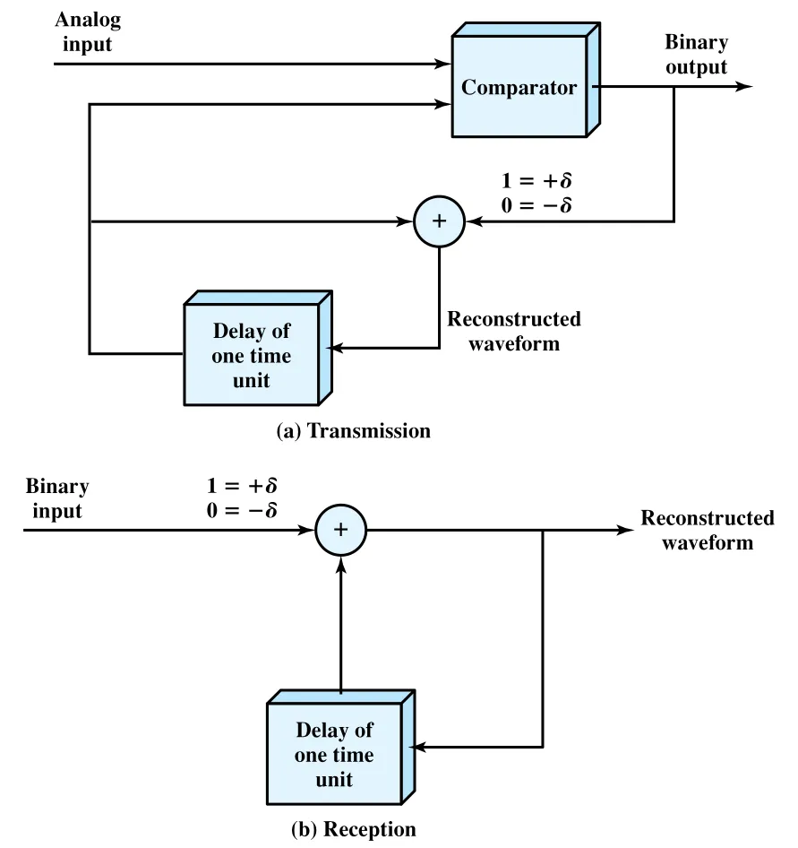 Figure 5.21 · PDF p. 186 · delta modulation의 송신 feedback loop와 수신 재구성 구조
DM의 핵심 parameter는 step size 와 sampling rate다. 가 너무 크면 waveform이 천천히 변할 때 staircase가 세밀하게 따라가지 못해 quantizing noise가 커진다. 가 너무 작으면 waveform이 빠르게 변할 때 staircase가 기울기를 따라가지 못해 slope overload noise가 커진다. sampling rate를 높이면 정확도는 좋아지지만 output data rate가 증가한다.
PCM과 비교하면 DM의 장점은 implementation simplicity다. 같은 data rate에서는 일반적으로 PCM이 더 좋은 SNR characteristic을 보인다.
Analog-to-Digital 성능 관점
voice를 PCM으로 재현하려면 7-bit coding, 즉 128 quantization levels 정도로도 좋은 품질을 얻을 수 있다. voice bandwidth를 4 kHz로 보면 sampling theorem에 따라 8000 samples/second가 필요하므로 data rate는 kbps가 된다. 반면 original analog voice signal은 4 kHz bandwidth만 차지한다. PCM으로 digital signal을 만들면 Nyquist criterion상 대략 28 kHz 정도의 bandwidth가 필요할 수 있다.
그럼에도 analog data를 digital signal로 바꾸는 방식이 널리 쓰이는 이유는 다음과 같다.
- repeater를 사용할 수 있어 amplifier처럼 cumulative noise를 계속 키우지 않는다.
- digital signal에는 TDM(Time Division Multiplexing)을 쓰기 좋고, analog FDM(Frequency Division Multiplexing)의 intermodulation noise 문제를 피할 수 있다.
- digital switching technique을 사용할 수 있다.
마지막으로 실제 telecommunication network에서는 digital-to-analog와 analog-to-digital conversion이 여러 번 섞일 수 있다. user terminal의 digital data가 modem에서 analog signal로 바뀌고, network 내부에서 codec으로 digitized되었다가 다시 여러 변환을 겪을 수 있다. 또한 voice analog signal과 digital data를 analog encoding한 signal은 spectrum 특성이 다르다. analog-encoded digital signal은 high-frequency component가 더 고르게 포함되므로, 이를 digitize할 때는 DM보다 PCM-related technique이 더 적합한 경우가 많다.
5.4 Analog Data, Analog Signals
Analog data를 analog signal로 보낼 때도 modulation이 필요할 수 있다. voice signal은 telephone line에서 baseband transmission으로 직접 보낼 수 있지만, 모든 경우에 baseband가 적합한 것은 아니다. analog modulation을 쓰는 주요 이유는 두 가지다.
- unguided transmission에서는 effective transmission을 위해 더 높은 frequency가 필요하다. baseband signal을 그대로 방사하려면 antenna가 비현실적으로 커질 수 있다.
- modulation은 FDM(Frequency Division Multiplexing)을 가능하게 한다. 여러 signal을 spectrum의 서로 다른 위치로 옮겨 같은 transmission medium을 공유할 수 있다.
Analog data의 주요 analog modulation 방식은 AM(Amplitude Modulation), FM(Frequency Modulation), PM(Phase Modulation)이다.
Amplitude Modulation (AM)
AM은 carrier의 amplitude를 input analog signal에 따라 변화시키는 가장 단순한 modulation이다. 원문은 AM을 다음처럼 표현한다.
여기서 는 unity amplitude로 normalized된 input signal, 는 modulation index, 는 carrier다. 는 input signal amplitude와 carrier amplitude의 비율이다. 식의 1은 dc component로, envelope가 원래 signal 정보를 잃지 않도록 해준다. 이 방식은 DSBTC(Double Sideband Transmitted Carrier)라고도 한다.
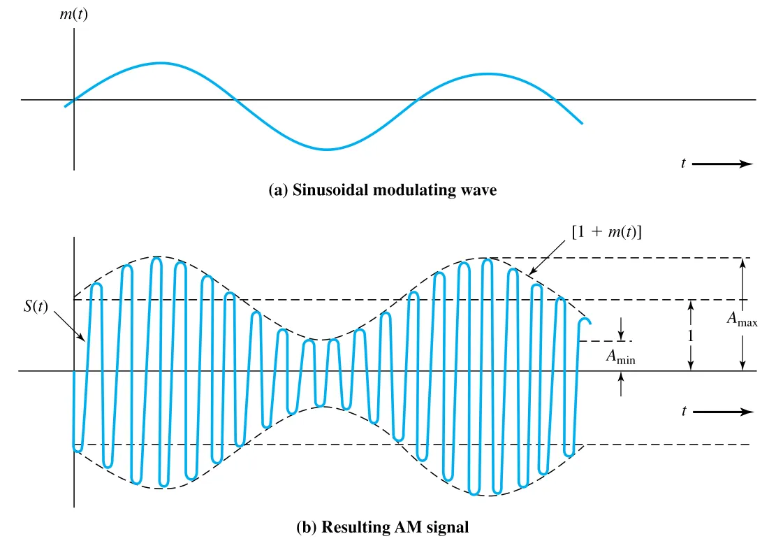 Figure 5.22 · PDF p. 189 · sinusoidal modulating wave가 AM signal envelope로 나타나는 모습
AM에서 envelope는 다. 이면 envelope가 original signal을 정확히 나타내지만, 이면 envelope가 time axis를 cross하면서 information이 손실된다. 따라서 modulation index는 크게 하고 싶지만 1을 넘기면 안 된다.
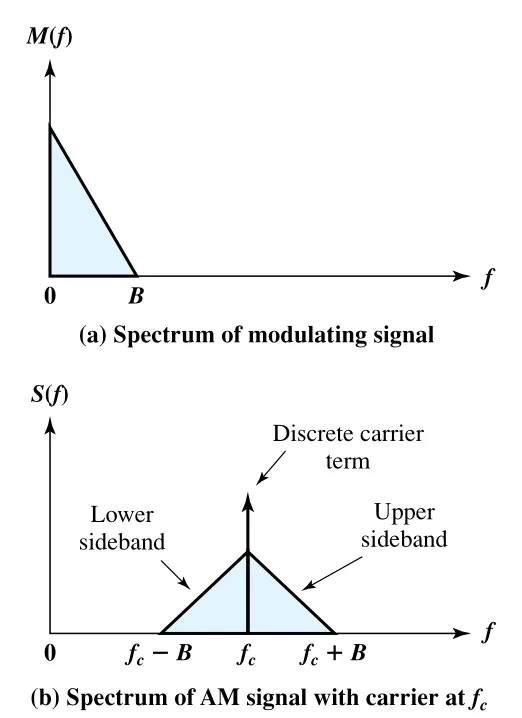 Figure 5.23 · PDF p. 189 · AM signal의 carrier, lower sideband, upper sideband spectrum
AM spectrum은 original carrier와 input signal spectrum이 carrier frequency 주변으로 이동한 sideband들로 구성된다. 보다 높은 쪽은 upper sideband, 낮은 쪽은 lower sideband다. 두 sideband는 모두 original spectrum 의 replica이고, lower sideband는 frequency-reversed 형태다. 예를 들어 300-3000 Hz voice signal을 60 kHz carrier에 modulation하면 upper sideband는 60.3-63 kHz, lower sideband는 57-59.7 kHz, carrier는 60 kHz에 생긴다.
AM total transmitted power는 다음 관계로 설명된다.
여기서 는 carrier power다. 정보 전달에 더 많은 power를 쓰려면 를 크게 하고 싶지만, 는 1보다 작아야 한다.
AM signal에는 중복이 많다. 각 sideband가 의 complete spectrum을 담고 있기 때문이다. SSB(Single Sideband)는 한 sideband만 보내고 다른 sideband와 carrier를 제거한다. 장점은 bandwidth가 로 줄어 DSBTC의 보다 절반이고, carrier와 다른 sideband에 power를 쓰지 않아 전력도 줄어든다는 점이다. DSBSC(Double Sideband Suppressed Carrier)는 carrier만 제거하고 두 sideband를 보내므로 power는 아끼지만 bandwidth는 DSBTC와 같다. VSB(Vestigial Sideband)는 한 sideband와 reduced-power carrier를 사용하는 compromise다. carrier를 억제하면 synchronization 단서가 줄어들 수 있기 때문이다.
Angle Modulation: FM과 PM
FM과 PM은 모두 angle modulation의 special case다.
PM(Phase Modulation)에서는 instantaneous phase deviation 가 modulating signal 에 비례한다.
FM(Frequency Modulation)에서는 phase의 derivative, 즉 instantaneous frequency deviation이 에 비례한다.
frequency는 phase의 변화율이므로, FM은 “phase 자체”가 아니라 “phase가 얼마나 빨리 변하는가”를 data에 맞춰 바꾸는 방식으로 이해할 수 있다.
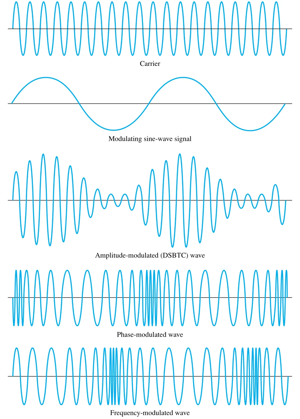 Figure 5.24 · PDF p. 192 · 같은 sine-wave carrier에 AM, PM, FM을 적용했을 때 waveform 비교
Figure 5.24에서 AM은 amplitude envelope가 변하고, PM과 FM은 amplitude는 일정하지만 zero crossing 간격과 phase progression이 변한다. FM과 PM waveform은 모양만 보고는 구분하기 어려우며, 어떤 modulation function을 사용했는지 알아야 한다.
AM과 angle modulation의 차이는 bandwidth와 power에서 드러난다. AM은 linear process라 carrier와 modulating signal의 sum/difference frequency를 만들며, bandwidth는 다. 반면 angle modulation은 nonlinear term을 포함하므로 , 등 더 넓은 frequency component를 만든다. 이론적으로는 infinite bandwidth가 필요하지만, 실무적으로는 Carson’s rule을 쓴다.
FM에서는 다음처럼도 쓸 수 있다.
여기서 는 peak frequency deviation이다. 따라서 FM과 PM은 일반적으로 AM보다 더 큰 bandwidth를 요구한다. 대신 FM에서 modulation magnitude가 커져 가 증가해도 average power level은 로 유지된다. 이는 modulation level이 AM signal power에 영향을 주지만 bandwidth에는 직접 영향을 주지 않는 AM과 대비된다.
연결 관계
이 장의 네 조합은 physical layer에서 “data representation”과 “signal propagation”을 연결한다. Chapter 3의 bandwidth, noise, BER, , Nyquist criterion은 여기서 line code와 modulation scheme의 성능 비교 기준으로 다시 등장한다. Chapter 4의 transmission media 관점에서는 guided media든 unguided media든 매체가 허용하는 frequency range와 propagation 특성에 맞춰 signal form을 골라야 한다.
Digital-to-digital encoding은 주로 baseband digital transmission 문제다. NRZ는 단순하고 bandwidth 효율적이지만 synchronization과 dc component가 문제다. Manchester와 Differential Manchester는 self-clocking을 얻는 대신 higher signaling rate를 요구한다. AMI, B8ZS, HDB3는 dc component를 줄이고 synchronization을 유지하면서 long-distance/high data rate transmission에 맞춘 compromise다.
Digital-to-analog modulation은 modem, wireless, optical signaling처럼 digital data를 carrier 기반 analog signal에 실어야 할 때 등장한다. ASK/FSK/PSK는 carrier의 amplitude/frequency/phase 중 무엇을 바꾸는지로 구분되고, QPSK/QAM은 signal element 하나에 여러 bit를 담아 bandwidth efficiency를 높인다. 다만 state 수가 늘수록 noise margin은 줄어든다.
Analog-to-digital conversion은 voice/video를 digital network에서 다루기 위한 관문이다. PCM은 sampling, quantization, encoding으로 analog waveform을 bit stream으로 바꾸고, companding으로 low-amplitude signal의 relative distortion을 줄인다. DM은 단순하지만 step size와 sampling rate가 quantizing noise와 slope overload noise를 동시에 좌우한다.
Analog-to-analog modulation은 baseband analog signal을 higher frequency band로 이동시켜 unguided transmission이나 FDM에 맞춘다. AM은 linear하고 bandwidth 해석이 단순하지만 carrier/sideband 중복이 있다. FM/PM은 angle modulation으로 일반적으로 bandwidth를 더 많이 쓰지만 amplitude가 일정하고, modulation magnitude가 power보다는 bandwidth에 영향을 준다.
오해하기 쉬운 내용
- bit rate와 baud는 같지 않다. bit rate 은 data element 속도이고, baud 는 signal element 속도다. QPSK나 QAM처럼 symbol 하나가 여러 bit를 담으면 은 보다 클 수 있다.
- differential encoding은 “현재 level”이 아니라 “이전 symbol과의 변화”를 정보로 쓴다. NRZI, Differential Manchester, DPSK가 이 계열이다.
- Manchester는 synchronization이 뛰어나지만 공짜가 아니다. transition이 많아져 bandwidth requirement가 증가한다.
- multilevel signaling은 bandwidth efficiency를 높일 수 있지만 receiver가 더 많은 state를 구분해야 하므로 noise와 attenuation에 더 민감해질 수 있다.
- sampling theorem은 sample rate만 충분하면 analog sample에 정보가 들어 있다는 뜻이지, quantization 후에도 original signal을 완벽히 복원한다는 뜻은 아니다. quantizing noise는 별도로 생긴다.
- AM에서 modulation index를 크게 하면 정보 전달 power를 늘릴 수 있지만, 이면 envelope가 왜곡되어 information loss가 생긴다.
- FM과 PM은 waveform만 보고 쉽게 구분되지 않는다. PM은 phase deviation이 에 비례하고, FM은 frequency deviation, 즉 phase derivative가 에 비례한다.
면접 질문
- NRZ-L과 NRZI의 차이를 설명하고, NRZI가 polarity inversion에 강한 이유를 말해보라.
- Manchester encoding이 self-clocking code인 이유와 그 대가로 필요한 bandwidth 증가를 설명하라.
- Bipolar-AMI에서 긴 zero sequence가 문제인 이유와 B8ZS/HDB3가 이를 어떻게 해결하는지 설명하라.
- bit rate와 baud rate의 차이를 QPSK 또는 16-QAM 예로 설명하라.
- MFSK와 MPSK에서 증가가 bandwidth efficiency와 BER에 서로 반대로 작용하는 이유를 설명하라.
- PCM에서 sampling theorem, quantization, quantizing noise의 관계를 설명하라.
- companding이 low-amplitude voice signal에 유리한 이유를 설명하라.
- Delta Modulation에서 step size 를 크게/작게 잡을 때 각각 어떤 noise가 커지는지 설명하라.
- AM의 upper sideband/lower sideband와 SSB의 bandwidth 절감 원리를 설명하라.
- FM과 PM이 모두 angle modulation인 이유와 Carson’s rule이 필요한 이유를 설명하라.