Chapter 3. Growth of Functions

개요

Chapter 3는 알고리즘의 running time을 정확한 식이 아니라 입력 크기 n이 커질 때의 성장률(growth rate)로 다루는 방법을 정리한다. Chapter 2에서 insertion sort의 worst-case $\Theta(n^{2})$ 와 merge sort의 $\Theta(n \lg n)$ 을 비교했다면, 이 장은 그 표기법을 엄밀하게 정의하고, 알고리즘 분석에서 자주 등장하는 standard functions의 성질을 정리한다.

핵심 관점은 asymptotic efficiency다. 입력 크기가 충분히 커지면 exact running time의 multiplicative constants와 lower-order terms보다 input size 자체가 성능 차이를 지배한다. 따라서 asymptotically more efficient algorithm은 매우 작은 입력을 제외한 대부분의 입력에서 더 좋은 선택이 된다.

핵심 개념

용어	핵심 의미	검색 키워드
asymptotic efficiency	`n`이 무한히 커질 때 running time이 어떻게 증가하는지 보는 효율성	asymptotic efficiency
asymptotic notation	함수의 성장률을 constant factor와 충분히 큰 `n` 기준으로 비교하는 표기	asymptotic notation
Θ-notation	위아래 constant factor로 동시에 묶는 asymptotically tight bound	$\Theta(g(n)), tight bound$
O-notation	위쪽 constant factor bound, asymptotic upper bound	$O(g(n)), upper bound$
Ω-notation	아래쪽 constant factor bound, asymptotic lower bound	$\Omega(g(n)), lower bound$
o-notation	어떤 constant factor로도 위에서 엄격히 작아지는 asymptotic upper bound	o(g(n)), strictly smaller
ω-notation	어떤 constant factor로도 아래에서 엄격히 커지는 asymptotic lower bound	$\omega(g(n)), strictly larger$
asymptotically nonnegative	충분히 큰 `n`에서 0 이상인 함수	asymptotically nonnegative

세부 정리

3.1 Asymptotic notation

왜 exact running time을 버리는가

정확한 running time을 구할 수 있는 경우도 있지만, 보통 그 정밀도는 계산 노력에 비해 큰 이득을 주지 않는다. Chapter 2의 insertion sort 분석처럼 $an^{2} + bn + c$ 같은 식을 얻어도, 충분히 큰 입력에서는 lower-order terms와 constant factor보다 최고차 성장률이 더 중요하다.

이때 우리가 보는 것은 algorithm의 asymptotic efficiency다. 이는 input size가 bound 없이 커질 때 running time이 어떤 비율로 증가하는지에 관한 성질이다. 예를 들어 $\Theta(n \lg n)$ merge sort는 $\Theta(n^{2})$ insertion sort보다 충분히 큰 입력에서 asymptotically more efficient하다.

Asymptotic notation은 function에 적용된다

CLRS는 asymptotic notation을 알고리즘의 running time을 표현하는 데 주로 사용하지만, 엄밀히는 notation이 function에 적용된다고 설명한다. INSERTION-SORT의 worst-case running time을 $an^{2} + bn + c$ 로 나타낸 뒤 $\Theta(n^{2})$ 라고 쓰는 것은, 그 running-time function이 $\Theta(n^{2})$ 에 속한다는 뜻이다.

따라서 asymptotic notation은 running time뿐 아니라 space usage나 알고리즘과 무관한 수학적 function에도 적용될 수 있다. 또한 running time에 적용할 때도 “worst-case running time”인지, “모든 input에 대한 blanket statement”인지 구분해야 한다.

기본 정의의 domain은 natural numbers $N = {0, 1, 2, \ldots}$ 다. 이는 input size가 보통 정수이기 때문이다. 다만 실제 분석에서는 real numbers로 확장하거나 natural numbers의 subset에 제한하는 식의 abuse를 할 때가 있다. CLRS의 태도는 “abuse는 하되 misuse는 하지 말자”에 가깝다. 즉 표기의 정확한 뜻을 알고 편의상 확장해야 한다.

Θ-notation: asymptotically tight bound

$\Theta(g(n))$ 은 $g(n)$ 과 같은 성장률을 constant factor 범위 안에서 갖는 함수들의 집합이다.

\begin{aligned} \Theta(g(n)) = \left\{ f(n) : \begin{array}{l} \text{there exist positive constants } c_1, c_2, \text{ and } n_0 \\ \text{such that } 0 \le c_1 g(n) \le f(n) \le c_2 g(n) \\ \text{for all } n \ge n_0 \end{array} \right\} \end{aligned}

즉 충분히 큰 $n$ 부터 $f(n)$ 이 $c_1 g(n)$ 과 $c_2 g(n)$ 사이에 끼어 있으면 $f(n) = \Theta(g(n))$ 라고 쓴다. 엄밀히는 $f(n) \in \Theta(g(n))$ 가 맞지만, CLRS는 관례적으로 $f(n) = \Theta(g(n))$ 라고 쓴다. 여기서 $g(n)$ 은 $f(n)$ 의 asymptotically tight bound다.

Figure 3.1은 Θ, O, Ω의 직관을 한 그림에 모아 보여준다. Θ는 위와 아래에서 동시에 묶는 tight bound이고, O는 위쪽 bound, Ω는 아래쪽 bound다.

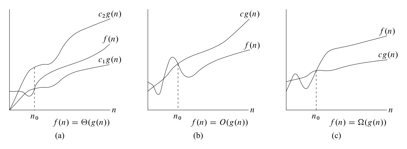Figure 3.1 · PDF p. 66 · Θ, O, Ω notation의 constant-factor bound 직관

정의에서 중요한 조건은 $n_0$ 이후만 본다는 점이다. $n < n_0$ 에서 함수들이 어떻게 움직이는지는 asymptotic bound에 영향을 주지 않는다. 또한 $c_1$ , $c_2$ , $n_0$ 는 하나로 고정된 “정답”이 아니라 존재하기만 하면 된다. 더 큰 $n_0$ 나 다른 constants도 가능하다.

Asymptotically nonnegative 조건

$\Theta(g(n))$ 의 정의는 $0 \le c_1 g(n) \le f(n) \le c_2 g(n)$ 형태를 갖기 때문에, $f(n)$ 은 충분히 큰 $n$ 에서 nonnegative여야 한다. 이를 asymptotically nonnegative라고 한다. 충분히 큰 $n$ 에서 positive이면 asymptotically positive function이다.

결과적으로 $g(n)$ 도 asymptotically nonnegative여야 $\Theta(g(n))$ 이 비어 있지 않다. CLRS는 이후 이 장의 모든 asymptotic notation 안에 들어가는 함수가 asymptotically nonnegative라고 가정한다.

Lower-order terms와 leading coefficient를 무시해도 되는 이유

Chapter 2의 비공식 규칙, 즉 lower-order terms를 버리고 leading coefficient를 무시한다는 직관은 Θ의 formal definition으로 정당화된다. 예를 들어

(1/2)n^{2} - 3n = \Theta(n^{2})

임을 보이려면 positive constants $c_1$ , $c_2$ , $n_0$ 가 존재해

c_1 n^{2} \le (1/2)n^{2} - 3n \le c_2 n^{2}

가 모든 $n \ge n_0$ 에서 성립함을 보이면 된다. 원문은 $c_1 = 1/14$ , $c_2 = 1/2$ , $n_0 = 7$ 같은 선택이 가능하다고 보인다. 중요한 것은 특정 constants가 유일하다는 점이 아니라, 어떤 적절한 constants가 존재한다는 점이다.

반대로 $6n^{3}$ 은 $\Theta(n^{2})$ 가 아니다. 만약 $6n^{3} \le c_2 n^{2}$ 가 충분히 큰 모든 $n$ 에서 성립해야 한다면, 나누어서 $n \le c_2/6$ 이 되어야 한다. 하지만 $c_2$ 는 constant이므로 임의로 큰 $n$ 에 대해 성립할 수 없다.

일반적으로 최고차항 계수가 양수인 polynomial

p(n) = \sum_{i=0}^{d} a_i n^{i}, \quad a_d > 0

은 $p(n) = \Theta(n^{d})$ 다. Constant function은 degree 0 polynomial이므로 $\Theta(n^{0})$ , 즉 흔히 $\Theta(1)$ 로 쓴다.

O-notation: asymptotic upper bound

$\Theta$ -notation이 함수의 위와 아래를 동시에 묶는다면, $O$ -notation은 위쪽 bound만 준다. $O(g(n))$ 은 충분히 큰 $n$ 에서 $f(n)$ 이 $g(n)$ 의 어떤 constant multiple 이하로 제한되는 함수들의 집합이다.

\begin{aligned} O(g(n)) = \left\{ f(n) : \begin{array}{l} \text{there exist positive constants } c \text{ and } n_0 \\ \text{such that } 0 \le f(n) \le c g(n) \\ \text{for all } n \ge n_0 \end{array} \right\} \end{aligned}

$f(n) = \Theta(g(n))$ 이면 반드시 $f(n) = O(g(n))$ 이다. 즉 $\Theta(g(n)) ⊆ O(g(n))$ 이다. 하지만 반대는 일반적으로 성립하지 않는다. 예를 들어 $n = O(n^{2})$ 는 맞지만 $n = \Theta(n^{2})$ 는 아니다.

CLRS는 O-notation을 asymptotically tight bound로 쓰지 않는다. 일부 문헌에서는 O를 느슨하게 “대략 그 정도”로 쓰지만, 이 책에서 $f(n) = O(g(n))$ 은 오직 $g(n)$ 의 constant multiple이 $f(n)$ 의 asymptotic upper bound라는 주장일 뿐이다. Tightness를 말하려면 $\Theta$ 를 써야 한다.

O-notation은 알고리즘 구조만 보고 빠르게 upper bound를 잡을 때 유용하다. 예를 들어 insertion sort의 double nested loop 구조만 봐도 inner loop의 각 iteration cost는 $O(1)$ 이고, i, j 조합은 최대 $n^{2}$ 개이므로 worst-case running time이 $O(n^{2})$ 임을 바로 알 수 있다.

Running time을 O로 말할 때의 의미

“Insertion sort의 running time은 $O(n^{2})$ 이다”라는 문장은 엄밀히는 약간의 abuse다. 같은 size n의 input이라도 실제 running time은 입력 상태에 따라 달라지기 때문이다. 이 문장의 정확한 뜻은 다음과 같다.

모든 size n의 input에 대해 실제 running time을 위에서 제한하는 어떤 function $f(n) = O(n^{2})$ 가 존재한다.

동치로 말하면 worst-case running time이 $O(n^{2})$ 이라는 뜻이다. 따라서 worst-case에 대한 O bound는 모든 input에 대한 blanket upper bound를 준다.

반면 “insertion sort의 worst-case running time은 $\Theta(n^{2})$ ”라는 말은 “모든 input에서 $\Theta(n^{2})$ 가 걸린다”는 뜻이 아니다. 이미 정렬된 input에서는 insertion sort가 $\Theta(n)$ 에 실행된다.

Ω-notation: asymptotic lower bound

Ω-notation은 O-notation의 반대 방향이다. $\Omega(g(n))$ 은 충분히 큰 n에서 $f(n)$ 이 $g(n)$ 의 어떤 positive constant multiple 이상인 함수들의 집합이다.

\begin{aligned} \Omega(g(n)) = \left\{ f(n) : \begin{array}{l} \text{there exist positive constants } c \text{ and } n_0 \\ \text{such that } 0 \le c g(n) \le f(n) \\ \text{for all } n \ge n_0 \end{array} \right\} \end{aligned}

$\Omega$ 는 lower bound다. 알고리즘의 running time에 modifier 없이 “ $\Omega(g(n))$ 이다”라고 말하면, 어떤 size n input을 골라도 running time이 충분히 큰 n에서 $g(n)$ 의 constant multiple 이상이라는 뜻이다. 동치로 best-case running time에 대한 lower bound다.

Insertion sort의 running time은 $\Omega(n)$ 이면서 $O(n^{2})$ 이다. 모든 input에서 적어도 linear 정도는 필요하지만, 모든 input에서 quadratic이라고 말할 수는 없다. 다만 worst-case running time은 $\Omega(n^{2})$ 라고 말할 수 있다. worst-case를 만드는 input, 즉 reverse sorted input이 존재하기 때문이다.

Theorem 3.1: Θ는 O와 Ω의 교집합

Theorem 3.1은 세 표기의 관계를 명확히 한다.

f(n) = \Theta(g(n)) iff f(n) = O(g(n)) and f(n) = \Omega(g(n))

즉 asymptotically tight bound를 보이려면 upper bound와 lower bound를 함께 보이면 된다. 실제 증명에서는 $\Theta$ 를 먼저 보인 뒤 O, $\Omega$ 를 얻기보다, O와 $\Omega$ 를 각각 증명한 뒤 Theorem 3.1로 $\Theta$ 를 결론내리는 경우가 많다.

Asymptotic notation in equations and inequalities

CLRS는 asymptotic notation을 equation 안에서도 사용한다. 이때 표기는 함수 집합을 나타내기도 하고, 이름 붙이지 않은 anonymous function을 나타내기도 한다.

$n = O(n^{2})$ 처럼 asymptotic notation이 오른쪽에 단독으로 있으면, equal sign은 set membership을 뜻한다.

n = O(n^{2}) means n \in O(n^{2})

반면 더 큰 식 안에 나타나면, asymptotic notation은 이름 붙이지 않은 어떤 함수를 뜻한다.

2n^{2} + 3n + 1 = 2n^{2} + \Theta(n)

이 식은 3n + 1을 어떤 $f(n) \in \Theta(n)$ 로 보아 $2n^{2} + f(n)$ 이라고 쓴 것이다. 이 방식은 recurrence에서 lower-order detail을 숨기는 데 유용하다. 예를 들어 merge sort recurrence

T(n) = 2T(n/2) + \Theta(n)

에서 $\Theta(n)$ 은 divide와 combine에 드는 linear amount of work를 나타내는 anonymous function이다.

Asymptotic notation이 왼쪽에 나타나면 규칙이 조금 다르다.

2n^{2} + \Theta(n) = \Theta(n^{2})

이 문장은 왼쪽의 anonymous function을 어떻게 골라도, 오른쪽의 anonymous function을 적절히 골라 등식이 성립하게 할 수 있다는 뜻이다. 즉 오른쪽이 왼쪽보다 더 coarse한 수준의 detail을 제공한다.

따라서 다음과 같은 chaining도 가능하다.

\begin{aligned} 2n^{2} + 3n + 1 &= 2n^{2} + \Theta(n) \\ &= \Theta(n^{2}) \end{aligned}

직관적으로는 lower-order term을 먼저 $\Theta(n)$ 로 뭉개고, 다시 전체를 $\Theta(n^{2})$ 로 뭉갠 것이다.

o-notation: non-tight upper bound

$O$ upper bound는 tight할 수도 있고 아닐 수도 있다. $2n^{2} = O(n^{2})$ 는 tight하지만, $2n = O(n^{2})$ 는 tight하지 않다. 이런 “엄격히 더 작은 성장률”을 나타내기 위해 $o$ -notation을 쓴다.

\begin{aligned} o(g(n)) = \left\{ f(n) : \begin{array}{l} \text{for any positive constant } c > 0, \\ \text{there exists a constant } n_0 > 0 \\ \text{such that } 0 \le f(n) < c g(n) \\ \text{for all } n \ge n_0 \end{array} \right\} \end{aligned}

$O$ 에서는 어떤 constant $c$ 하나만 찾으면 되지만, $o$ 에서는 모든 positive constant $c$ 에 대해 결국 $f(n) < c g(n)$ 이 되어야 한다. 즉 $f(n)$ 이 $g(n)$ 에 비해 asymptotically insignificant해진다.

\begin{aligned} 2n &= o(n^{2}) \\ 2n^{2} &\ne o(n^{2}) \end{aligned}

Limit이 존재한다면 $f(n) = o(g(n))$ 은 다음과 같은 직관과 대응한다.

lim_{n \to \infty} f(n) / g(n) = 0

ω-notation: non-tight lower bound

ω-notation은 Ω-notation에 대한 strict version이다. $f(n)$ 이 $g(n)$ 보다 asymptotically larger하다는 뜻이다.

\begin{aligned} \omega(g(n)) = \left\{ f(n) : \begin{array}{l} \text{for any positive constant } c > 0, \\ \text{there exists a constant } n_0 > 0 \\ \text{such that } 0 \le c g(n) < f(n) \\ \text{for all } n \ge n_0 \end{array} \right\} \end{aligned}

예를 들어 $n^{2} / 2 = \omega(n)$ 이지만, $n^{2} / 2 \ne \omega(n^{2})$ 이다. Limit이 존재하면 다음 직관과 대응한다.

lim_{n \to \infty} f(n) / g(n) = \infty

Comparing functions

Asymptotic comparisons는 real number comparison과 비슷한 성질을 많이 가진다. 아래 성질들은 $f(n)$ , $g(n)$ , $h(n)$ 이 asymptotically positive라고 가정할 때 사용한다.

성질	적용되는 표기	의미
transitivity	$\Theta$ , `O`, $\Omega$ , `o`, $\omega$	`f`가 `g`에 대해, `g`가 `h`에 대해 같은 관계면 `f`와 `h`도 그 관계다
reflexivity	$\Theta$ , `O`, $\Omega$	$f(n)$ 은 자기 자신에 대해 tight/upper/lower bound다
symmetry	$\Theta$	$f = \Theta(g)$ iff $g = \Theta(f)$
transpose symmetry	$O$ 와 $\Omega$ , $o$ 와 $\omega$	$f = O(g)$ iff $g = \Omega(f)$ , $f = o(g)$ iff $g = \omega(f)$

실수 비교와의 비유는 다음과 같다.

Asymptotic comparison	Real-number analogy
$f(n) = O(g(n))$	$a \le b$
$f(n) = \Omega(g(n))$	$a \ge b$
$f(n) = \Theta(g(n))$	$a = b$
$f(n) = o(g(n))$	$a < b$
$f(n) = \omega(g(n))$	$a > b$

하지만 trichotomy는 함수 비교에 그대로 적용되지 않는다. 실수 $a$ , $b$ 는 반드시 $<$ , $=$ , $>$ 중 하나지만, 함수는 asymptotically incomparable할 수 있다. 원문 예시는 $n$ 과 $n^{1 + \sin n}$ 이다. $\sin n$ 때문에 exponent가 0과 2 사이를 oscillate하므로, 어느 한쪽이 항상 asymptotic upper/lower bound라고 말하기 어렵다.

3.2 Standard notations and common functions

Monotonicity

함수의 단조성(monotonicity)은 알고리즘 분석에서 recurrence, summation bound, search space 감소를 다룰 때 자주 쓰인다.

용어	정의
monotonically increasing	$m \le n$ 이면 $f(m) \le f(n)$
monotonically decreasing	$m \le n$ 이면 $f(m) \ge f(n)$
strictly increasing	$m < n$ 이면 $f(m) < f(n)$
strictly decreasing	$m < n$ 이면 $f(m) > f(n)$

예를 들어 $n^{a}$ 는 $a \ge 0$ 이면 monotonically increasing이고, $a \le 0$ 이면 monotonically decreasing이다. Logarithm $\log_b n$ 은 base $b > 1$ 이 고정되어 있으면 $n > 0$ 에서 strictly increasing이다.

Floors and ceilings

Floor와 ceiling은 array index, divide-and-conquer split, recurrence에서 정수 크기를 다룰 때 필요하다.

표기	의미
$\lfloor x \rfloor$	$x$ 이하의 가장 큰 integer, floor of $x$
$\lceil x \rceil$	$x$ 이상의 가장 작은 integer, ceiling of $x$

기본 부등식은 다음과 같다.

x - 1 < \lfloor x \rfloor \le x \le \lceil x \rceil < x + 1

정수 $n$ 에 대해서는

\lceil n/2 \rceil + \lfloor n/2 \rfloor = n

이므로 merge sort처럼 array를 반으로 나눌 때 두 subproblem size가 정확히 합쳐져 원래 크기가 된다. Floor function과 ceiling function은 모두 monotonically increasing이다.

CLRS는 nested floor/ceiling을 단순화하는 식도 제공한다. 알고리즘 분석에서는 정확한 정수 반올림보다 “상수 차이 안에서 같은 성장률”이 중요한 경우가 많지만, recurrence를 엄밀히 다룰 때 $\lceil \lceil x/a \rceil/b \rceil = \lceil x/(ab) \rceil$ , $\lfloor \lfloor x/a \rfloor/b \rfloor = \lfloor x/(ab) \rfloor$ 같은 성질이 유용하다.

Modular arithmetic

Modular arithmetic은 hashing, number-theoretic algorithms, cryptography에서 기본이 된다. 정수 $a$ 와 positive integer $n$ 에 대해

\begin{aligned} a \bmod n &= a - n\lfloor a/n \rfloor \\ 0 &\le a \bmod n < n \end{aligned}

이다. 두 정수 $a$ , $b$ 의 remainder가 같으면

a \equiv b \pmod n

이라고 쓰고, $a$ is equivalent to $b$ , modulo $n$ 이라고 읽는다. 동치 조건은 $n$ 이 $b - a$ 를 나눈다는 것이다. 같지 않으면 $a \not\equiv b \pmod n$ 이라고 표현한다.

Polynomials

Degree $d$ 의 polynomial은 다음 형태의 함수다.

p(n) = \sum_{i=0}^{d} a_i n^{i}, \quad a_d \ne 0

$a_0, a_1, \ldots, a_d$ 는 coefficients이고, $a_d$ 는 leading coefficient다. Polynomial이 asymptotically positive인 것은 $a_d > 0$ 일 때와 정확히 대응한다. 이 경우

p(n) = \Theta(n^{d})

이다. 즉 알고리즘 분석에서 polynomial의 성장률은 최고차항의 degree가 결정한다.

함수 $f(n)$ 이 어떤 constant $k$ 에 대해 $O(n^{k})$ 이면 polynomially bounded라고 한다. 이 표현은 “다항식 정도로 제한되는 성장”을 말할 때 자주 쓰이며, exponential이나 factorial과 대비된다.

Exponentials

Exponential functions는 polynomial보다 훨씬 빠르게 성장한다. 기본 항등식은 다음과 같다.

\begin{aligned} a^{0} &= 1 \\ a^{1} &= a \\ a^{-1} &= 1/a \\ (a^{m})^{n} &= a^{mn} \\ (a^{m})^{n} &= (a^{n})^{m} \\ a^{m} a^{n} &= a^{m+n} \end{aligned}

$a \ge 1$ 이면 $a^{n}$ 은 $n$ 에 대해 monotonically increasing이다. 편의상 $0^{0} = 1$ 로 가정할 때도 있다.

Polynomial과 exponential의 성장률 관계는 매우 중요하다. 모든 real constants $a > 1$ , $b$ 에 대해

\begin{aligned} \lim_{n \to \infty} n^{b} / a^{n} &= 0 \\ n^{b} &= o(a^{n}) \end{aligned}

이다. 즉 base가 1보다 큰 exponential function은 어떤 polynomial function보다도 asymptotically faster하게 성장한다.

자연상수 $e = 2.71828\ldots$ 는 natural logarithm의 base이며, 다음 급수로 정의된다.

e^{x} = \sum_{i=0}^{\infty} x^{i} / i!

자주 쓰는 부등식과 근사는 다음과 같다.

\begin{aligned} e^{x} &\ge 1 + x \quad \text{with equality only when } x = 0 \\ 1 + x &\le e^{x} \le 1 + x + x^{2} \quad \text{when } \lvert x \rvert \le 1 \\ e^{x} &= 1 + x + \Theta(x^{2}) \quad \text{as } x \to 0 \\ \lim_{n \to \infty} (1 + x/n)^{n} &= e^{x} \end{aligned}

여기서 $e^{x} = 1 + x + \Theta(x^{2})$ 의 asymptotic notation은 $n \to \infty$ 가 아니라 $x \to 0$ 에서의 limiting behavior를 설명한다. 이는 asymptotic notation이 본질적으로 “어떤 변수가 극한으로 갈 때의 함수 행동”을 나타낸다는 점을 보여준다.

Logarithms

CLRS의 logarithm notation은 다음과 같다.

표기	의미
$\lg n$	$\log_2 n$ , binary logarithm
$\ln n$	$\log_e n$ , natural logarithm
$\lg^{k} n$	$(\lg n)^{k}$ , exponentiation
$\lg \lg n$	$\lg(\lg n)$ , composition

중요한 convention은 logarithm이 다음 term에만 적용된다는 것이다. 따라서 $\lg n + k$ 는 $(\lg n) + k$ 이고 $\lg(n + k)$ 가 아니다.

Logarithm 항등식 중 특히 자주 쓰는 것은 base change다.

\log_{b} a = \log_{c} a / \log_{c} b

Base가 constant이면 logarithm base를 바꾸는 것은 constant factor만 바꾼다. 그래서 $O$ -notation이나 $\Theta$ -notation처럼 constant factor를 무시하는 맥락에서는 보통 $\lg n$ 을 대표 표기로 쓴다. Computer science에서 base 2가 자연스러운 이유는 많은 algorithms와 data structures가 problem을 two parts로 나누기 때문이다.

그 밖의 기본 항등식은 다음과 같다.

\begin{aligned} \log_{c}(ab) &= \log_{c} a + \log_{c} b \\ \log_{b}(a^{n}) &= n \log_{b} a \\ \log_{b}(1/a) &= -\log_{b} a \\ \log_{b} a &= 1 / \log_{a} b \\ a^{\log_{b} c} &= c^{\log_{b} a} \end{aligned}

$\ln(1 + x)$ 에는 $\lvert x\rvert < 1$ 에서의 series expansion이 있고, $x > -1$ 에 대해 다음 부등식이 사용된다.

x / (1 + x) \le \ln(1 + x) \le x

함수 $f(n)$ 이 어떤 constant $k$ 에 대해 $O(\lg^{k} n)$ 이면 polylogarithmically bounded라고 한다. Polynomial과 polylogarithm의 성장률 관계는 다음과 같다.

\lg^{b} n = o(n^{a}) \quad \text{for any constant } a > 0

즉 어떤 positive polynomial function도 어떤 polylogarithmic function보다 asymptotically faster하게 성장한다.

Factorials

Factorial function은 permutation 수, brute-force search space, combinatorial counting에서 자주 등장한다. 정수 $n \ge 0$ 에 대해

\begin{aligned} n! &= \begin{cases} 1, & \text{if } n = 0, \\ n(n - 1)!, & \text{if } n > 0. \end{cases} \end{aligned}

이며, 따라서 $n! = 1 \cdot 2 \cdot 3 \cdots n$ 이다. 약한 upper bound로는 각 항이 최대 $n$ 이므로

n! \le n^{n}

이 성립한다.

더 정밀한 근사는 Stirling’s approximation이다.

n! = \sqrt{2\pi n} (n/e)^{n} (1 + \Theta(1/n))

Stirling’s approximation으로 다음 성장률 관계를 얻는다.

\begin{aligned} n! &= o(n^{n}) \\ n! &= \omega(2^{n}) \\ \lg(n!) &= \Theta(n \lg n) \end{aligned}

즉 factorial은 $2^{n}$ 같은 fixed-base exponential보다 크지만, $n^{n}$ 보다는 작다. 또 $n!$ 자체는 매우 빠르게 커지지만 그 logarithm은 $n \lg n$ order다. 이 성질은 comparison sorting lower bound나 permutation counting에서 자주 연결된다.

Functional iteration

Functional iteration은 같은 함수를 반복 적용하는 표기다. $f^{(i)}(n)$ 은 초기값 $n$ 에 함수 $f$ 를 $i$ 번 적용한 결과다.

\begin{aligned} f^{(0)}(n) &= n \\ f^{(i)}(n) &= f(f^{(i-1)}(n)) if i > 0 \end{aligned}

예를 들어 $f(n) = 2n$ 이면

f^{(i)}(n) = 2^{i} n

이다. 이 표기는 iterated logarithm처럼 “몇 번 반복 적용해야 특정 threshold 아래로 내려가는가”를 표현할 때 중요하다.

Iterated logarithm: $\lg\cdot n$

Iterated logarithm $\lg\cdot n$ , 즉 log star of $n$ 은 $\lg$ 를 몇 번 반복 적용해야 값이 1 이하가 되는지를 나타낸다.

\lg^* n = \min \{ i \ge 0 : \lg^{(i)} n \le 1 \}

여기서 $\lg^{(i)} n$ 은 logarithm function을 $i$ 번 연속 적용한 것이고, $\lg^{i} n = (\lg n)^{i}$ 와 다르다. 이 둘을 혼동하면 안 된다.

대표 값은 다음과 같다.

n	$\lg\cdot n$
$2$	$1$
$4$	$2$
$16$	$3$
$65536$	$4$
$2^{65536}$	$5$

$\lg\cdot n$ 은 극도로 천천히 증가한다. 원문은 observable universe의 atom 수가 약 $10^{80}$ 이고 이것이 $2^{65536}$ 보다 훨씬 작으므로, 실제로 $\lg\cdot n > 5$ 인 input size를 거의 만나지 않는다고 설명한다.

Fibonacci numbers

Fibonacci numbers는 다음 recurrence로 정의된다.

\begin{aligned} F_0 &= 0 \\ F_1 &= 1 \\ F_i &= F_{i-1} + F_{i-2} \quad \text{for } i \ge 2 \end{aligned}

따라서 sequence는 다음과 같이 시작한다.

0, 1, 1, 2, 3, 5, 8, 13, 21, 34, 55, \ldots

Fibonacci numbers는 golden ratio $\phi$ 와 그 conjugate $\hat{\phi}$ 에 연결된다. 둘은 equation

x^{2} = x + 1

의 두 root다.

\begin{aligned} \phi &= (1 + \sqrt{5}) / 2 = 1.61803\ldots \\ \hat{\phi} &= (1 - \sqrt{5}) / 2 = -0.61803\ldots \end{aligned}

Fibonacci number의 closed form은 다음과 같다.

F_i = (\phi^{i} - \hat{\phi}^{i}) / \sqrt{5}

$\lvert \hat{\phi} \rvert < 1$ 이므로 $\hat{\phi}^{i} / \sqrt{5}$ 의 절댓값은 항상 $1/2$ 보다 작다. 따라서 $F_i$ 는 $\phi^{i} / \sqrt{5}$ 를 nearest integer로 반올림한 값이다.

F_i = \operatorname{floor}(\phi^{i} / \sqrt{5} + 1/2)

결론적으로 Fibonacci numbers grow exponentially. 이 성질은 naive recursive Fibonacci algorithm이 왜 지수적으로 느려지는지, 그리고 dynamic programming이나 memoization이 왜 효과적인지 설명하는 배경이 된다.

Exercises와 Problems가 요구하는 핵심 능력

Chapter 3의 exercises는 정의를 외우는 것보다, asymptotic notation을 정확히 조작하는 능력을 요구한다.

항목	핵심 능력
$\max(f(n), g(n)) = \Theta(f(n) + g(n))$	asymptotically nonnegative functions에서 sum과 max의 관계를 constants로 증명
$(n + a)^{b} = \Theta(n^{b})$	상수 shift가 polynomial growth를 바꾸지 않음을 증명
$2^{n+1}$ vs $2^{n}$ , $2^{2n}$ vs $2^{n}$	constant factor와 exponential factor 차이 구분
two-parameter notation $O(g(n,m))$	$n$ , $m$ 이 독립적으로 커질 때의 asymptotic bound 확장
relative asymptotic growths	$\lg^{k} n$ , $n^\varepsilon$ , $c^{n}$ , $n!$ , $\lg(n!)$ 같은 함수군 순서 비교
asymptotic notation properties	$O$ , $\Omega$ , $\Theta$ , $o$ , $\omega$ 의 참/거짓 명제를 반례나 정의로 판정
soft-oh `Õ`	logarithmic factors를 무시하는 변형 notation 이해
iterated functions	$\lg\cdot n$ 을 일반화해 어떤 함수 반복이 threshold까지 몇 번 필요한지 분석

특히 Problem 3-3의 ordering by asymptotic growth rates는 이 장의 종합 문제다. 함수들을 growth rate 순서로 정렬하고 $\Theta$ equivalence class로 묶는 훈련을 시킨다. 이 문제는 나중에 알고리즘 후보들의 running time을 비교할 때 “어느 항이 진짜 지배적인가”를 빠르게 판단하는 감각과 연결된다.

Chapter notes는 asymptotic notation의 역사적 배경도 짧게 언급한다. $O$ -notation은 Bachmann의 number theory text에서, $o$ -notation은 Landau의 prime distribution 논의에서 유래했고, $\Omega$ 와 $\Theta$ 는 $O$ 를 upper/lower/tight bound에 모두 쓰는 관행을 바로잡기 위해 Knuth가 강조한 표기다. 중요한 실전 포인트는 문헌마다 표기 정의가 약간 다를 수 있으므로, 어떤 의미의 $O$ , $\Omega$ , $\Theta$ 를 쓰는지 항상 문맥을 확인해야 한다는 점이다.

비교

Chapter 3의 growth hierarchy를 알고리즘 분석 관점에서 정리하면 다음과 같다. 아래로 갈수록 더 빠르게 증가하는 함수군이다.

성장률 계층	대표 예	핵심 관계
constant	$1$	input size와 무관
iterated logarithmic	$\lg\cdot n$	거의 모든 현실적 input에서 작은 상수처럼 보일 정도로 느림
logarithmic	$\lg n$ , $\ln n$	binary search, balanced tree height
polylogarithmic	$\lg^{k} n$	모든 positive polynomial보다 느림
polynomial	$n^{a}$ , $n$ , $n^{2}$ , $n^{3}$	$\lg^{k} n = o(n^{a})$ for $a > 0$
polynomial-log	$n \lg n$ , $\lg(n!)$	sorting lower bound, merge sort
exponential	$2^{n}$ , $c^{n}$	모든 polynomial보다 빠름
factorial	$n!$	permutation brute force, $\omega(2^{n})$ and $o(n^{n})$
super-exponential examples	$n^{n}$ , $2^{2^{n}}$	조합 폭발을 설명할 때 등장

자주 쓰는 비교식만 따로 모으면 다음과 같다.

\begin{aligned} \lg^{b} n &= o(n^{a}) \quad \text{for } a > 0 \\ n^{b} &= o(a^{n}) \quad \text{for } a > 1 \\ n! &= \omega(2^{n}) \\ n! &= o(n^{n}) \\ \lg(n!) &= \Theta(n \lg n) \\ F_i &= \Theta(\phi^{i}) \end{aligned}

연결 관계

Chapter 3는 이후 CLRS 전반의 분석 언어다. Chapter 4의 recurrences와 master theorem은 $\Theta$ , $O$ , $\Omega$ 로 결과를 표현한다. Sorting lower bound, dynamic programming table size, graph algorithm complexity, amortized analysis 모두 이 장의 notation과 function comparison을 계속 사용한다.

Chapter 2에서 $T(n) = 2T(n/2) + \Theta(n)$ 을 비공식적으로 다뤘다면, Chapter 3는 그 $\Theta(n)$ 이 anonymous function이고, exact lower-order terms를 숨기는 표기라는 점을 명확히 한다. Chapter 4 이후부터는 이 관례가 recurrence에 자연스럽게 들어간다.

또한 standard functions는 알고리즘 패턴과 연결된다. $\lg n$ 은 halving search나 balanced tree height, $n \lg n$ 은 divide-and-conquer sorting, $2^{n}$ 은 subset enumeration, $n!$ 은 permutation enumeration, $\lg\cdot n$ 은 극히 느리게 증가하는 반복 구조, Fibonacci growth는 naive recursion의 exponential blow-up과 연결된다.

오해하기 쉬운 내용

$O(g(n))$ 은 tight bound가 아니다. $n = O(n^{2})$ 는 참이지만 $n = \Theta(n^{2})$ 는 거짓이다.
“running time is $O(n^{2})$ ”는 보통 worst-case upper bound 또는 모든 input을 덮는 upper-bound function이 있다는 뜻이다.
“at least $O(n^{2})$ ” 같은 표현은 의미가 흐리다. 아래쪽 bound를 말하려면 $\Omega(n^{2})$ 를 써야 한다.
$\Theta(g(n))$ 는 $O(g(n))$ 와 $\Omega(g(n))$ 가 동시에 성립할 때다.
$o(g(n))$ 는 단순히 $O(g(n))$ 보다 작은 느낌이 아니라, 모든 constant factor보다 eventually 작아지는 strict upper bound다.
Asymptotic notation이 equation 안에 들어가면 anonymous function을 뜻할 수 있다. $2n^{2} + \Theta(n) = \Theta(n^{2})$ 는 일반 등호처럼 좌우 집합이 같다는 뜻이 아니다.
모든 함수 쌍이 asymptotically comparable한 것은 아니다. $n$ 과 $n^{1+\sin n}$ 처럼 oscillation이 있으면 $O$ 도 $\Omega$ 도 아닐 수 있다.
$\lg^{k} n$ 은 $(\lg n)^{k}$ 이고, $\lg^{(k)} n$ 은 logarithm을 k번 반복 적용한 것이다.
Logarithm base가 constant이면 asymptotic notation 안에서는 constant factor 차이만 만든다. 그래도 정확한 수식 변형에서는 base change를 명시해야 한다.
$\lg\cdot n$ 은 “log를 한 번 취한 값”이 아니라 “log를 몇 번 반복해야 1 이하가 되는가”를 나타내는 함수다.

면접 질문

$\Theta(g(n))$ , $O(g(n))$ , $\Omega(g(n))$ 의 formal definition을 constants $c$ , $c_1$ , $c_2$ , $n_0$ 를 사용해 설명하라.
$f(n) = \Theta(g(n))$ iff $f(n) = O(g(n))$ and $f(n) = \Omega(g(n))$ 인 이유를 설명하라.
왜 $n = O(n^{2})$ 는 참이지만 $n = \Theta(n^{2})$ 는 거짓인가?
Insertion sort의 worst-case running time이 $\Theta(n^{2})$ 인 것과 running time이 모든 input에서 $\Theta(n^{2})$ 라는 말의 차이를 설명하라.
o(g(n))와 $O(g(n))$ , $\omega(g(n))$ 와 $\Omega(g(n))$ 의 차이를 limit 관점에서 설명하라.
$2n^{2} + 3n + 1 = 2n^{2} + \Theta(n) = \Theta(n^{2})$ 같은 식을 어떻게 해석해야 하는가?
$\lg^{k} n$ 과 $\lg^{(k)} n$ 의 차이를 예시와 함께 설명하라.
왜 모든 positive polynomial은 polylogarithmic function보다 asymptotically faster하게 성장하는가?
왜 base가 1보다 큰 exponential function은 어떤 polynomial보다 빠르게 성장하는가?
Stirling’s approximation을 이용해 $\lg(n!) = \Theta(n \lg n)$ 이 되는 직관을 설명하라.
$\lg\cdot n$ 이 왜 현실적인 input size에서 거의 상수처럼 보이는지 설명하라.
Fibonacci numbers가 exponentially grow한다는 말이 naive recursive Fibonacci algorithm 분석과 어떻게 연결되는가?