Chapter 4. Divide-and-Conquer

개요

Chapter 4는 divide-and-conquer를 실제 알고리즘 설계와 recurrence 분석의 중심 도구로 확장한다. Chapter 2의 merge sort에서 본 Divide -> Conquer -> Combine 흐름을 다시 확인한 뒤, maximum-subarray problem, matrix multiplication, Strassen’s algorithm, substitution method, recursion-tree method, master method, master theorem proof까지 이어간다.

Divide-and-conquer algorithm은 recursive case와 base case를 함께 가진다. Recursive case에서는 문제를 같은 종류의 더 작은 subproblems로 나누고, subproblems를 재귀적으로 풀고, 결과를 combine한다. Base case에서는 subproblem이 충분히 작아져 더 이상 recursion하지 않고 straightforward하게 해결한다. 때때로 원래 문제와 정확히 같은 형태가 아닌 보조 subproblem을 풀어야 하는데, CLRS는 이를 보통 combine step의 일부로 본다.

핵심 개념

세부 정리

Recurrences and technicalities

Recurrence는 divide-and-conquer와 자연스럽게 따라다닌다. 어떤 algorithm이 size $n$ 문제를 더 작은 input에 대한 recursive calls로 풀면, running time $T(n)$도 더 작은 크기의 $T(\ldots)$를 포함하는 식으로 표현된다. 예를 들어 merge sort의 worst-case running time은 다음 recurrence로 표현된다.

Recurrence는 다양한 형태를 가질 수 있다. Unequal split이면 $T(n) = T(2n/3) + T(n/3) + \Theta(n)$처럼 되고, recursive linear search처럼 input을 하나만 줄이면 $T(n) = T(n - 1) + \Theta(1)$이 된다.

Chapter 4는 recurrence를 푸는 세 방법을 제시한다.

Recurrence를 쓸 때는 floors, ceilings, boundary conditions를 종종 생략한다. 예를 들어 실제 merge sort는 odd $n$에서 $T(\lceil n/2 \rceil) + T(\lfloor n/2 \rfloor) + \Theta(n)$이지만, 보통 $2T(n/2) + \Theta(n)$으로 쓴다. $T(1)$ 같은 작은 input의 정확한 값도 생략하는데, 이는 보통 exact solution만 constant factor만큼 바꾸고 asymptotic order는 바꾸지 않기 때문이다. 다만 이런 technicalities가 항상 무해한 것은 아니므로, 어떤 경우에 영향이 없는지 판단하는 감각이 필요하다.

4.1 The maximum-subarray problem

주식 매매 예시에서 maximum subarray로 변환하기

Maximum-subarray problem은 숫자 array에서 sum이 가장 큰 nonempty contiguous subarray를 찾는 문제다. CLRS는 Volatile Chemical Corporation 주식 예시로 시작한다. 미래 가격을 모두 안다고 할 때, 한 번 사고 나중에 한 번 팔아 profit을 최대화하고 싶다.

Figure 4.1은 17일 동안의 stock price와 daily change를 보여준다. 단순히 lowest price에 사고 highest price에 팔면 될 것 같지만, highest price가 lowest price보다 먼저 오면 불가능하다.

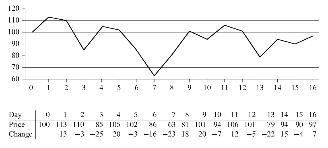Figure 4.1 · PDF p. 89 · 주식 가격과 전일 대비 change를 함께 보여 주는 maximum-subarray 예시

Figure 4.2는 maximum profit이 overall lowest price에서 시작하지도, overall highest price에서 끝나지도 않을 수 있음을 보여준다. 즉 문제는 단순히 전역 최소/최대 가격을 찾는 문제가 아니다.

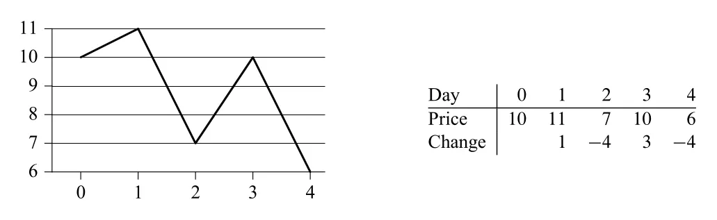Figure 4.2 · PDF p. 90 · maximum profit이 global minimum/maximum price 쌍으로 결정되지 않는 반례

핵심 변환은 price 자체가 아니라 daily change를 array $A$로 보는 것이다. Day $i$의 change는 day $i-1$ 종료 가격과 day $i$ 종료 가격의 차이다. 어떤 기간에 사고팔아 얻는 profit은 그 기간의 daily changes를 더한 값과 같다. 따라서 maximum profit은 daily-change array에서 maximum-sum contiguous subarray를 찾는 문제로 바뀐다.

Figure 4.3의 array에서는 $A[8..11] = <18, 20, -7, 12>$의 sum이 43으로 최대다. 이는 day 7 이후에 사고 day 11 이후에 팔면 주당 43달러 profit을 얻는다는 뜻이다.

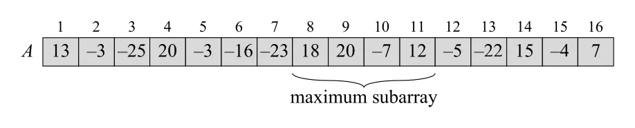Figure 4.3 · PDF p. 91 · daily change array에서 $A[8..11]$이 maximum subarray가 되는 예

Brute force와 문제의 성격

Brute-force solution은 모든 buy/sell date pair, 또는 모든 contiguous subarray를 검사한다. $n$일에 대해 가능한 pair는 $\Theta(n^{2})$개이고, subarray sums를 이전 계산값을 이용해 $O(1)$에 갱신하더라도 전체는 $\Theta(n^{2})$ time이다. 목표는 이를 $o(n^{2})$로 개선하는 것이다.

이 문제는 array에 negative numbers가 있을 때만 흥미롭다. 모든 entries가 nonnegative라면 전체 array가 maximum subarray이기 때문이다. 또한 maximum subarray가 여러 개 있을 수 있으므로 원문은 “the” maximum subarray보다 “a” maximum subarray라고 표현한다.

Divide-and-conquer 구조

$A[low..high]$의 maximum subarray를 찾는다고 하자. Midpoint $mid$를 기준으로 보면 어떤 contiguous subarray $A[i..j]$도 정확히 세 위치 중 하나에 속한다.

Figure 4.4는 이 세 위치와 crossing subarray의 구조를 보여준다. Crossing subarray는 반드시 $A[i..mid]$와 $A[mid+1..j]$의 결합이다.

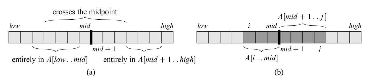Figure 4.4 · PDF p. 92 · maximum subarray가 left, right, crossing midpoint 중 하나에 속한다는 divide-and-conquer 구조

FIND-MAX-CROSSING-SUBARRAY

Crossing maximum subarray는 원래 problem의 smaller instance가 아니다. “반드시 midpoint를 crossing해야 한다”는 추가 제약이 있기 때문이다. 그래서 CLRS는 이를 combine step의 일부로 취급한다.

방법은 간단하다. Midpoint에서 왼쪽으로 내려가며 $A[i..mid]$ 중 최대 sum suffix를 찾고, $mid+1$에서 오른쪽으로 올라가며 $A[mid+1..j]$ 중 최대 sum prefix를 찾는다. 둘을 붙이면 maximum subarray crossing midpoint가 된다.

FIND-MAX-CROSSING-SUBARRAY(A, low, mid, high)
1  left-sum = -∞
2  sum = 0
3  for i = mid downto low
4      sum = sum + A[i]
5      if sum > left-sum
6          left-sum = sum
7          max-left = i
8  right-sum = -∞
9  sum = 0
10 for j = mid + 1 to high
11     sum = sum + A[j]
12     if sum > right-sum
13         right-sum = sum
14         max-right = j
15 return (max-left, max-right, left-sum + right-sum)

두 loops의 iteration 수는 $(mid - low + 1) + (high - mid) = high - low + 1 = n$이므로 running time은 $\Theta(n)$이다.

FIND-MAXIMUM-SUBARRAY

전체 recursive algorithm은 left, right, crossing 세 후보를 구한 뒤 sum이 가장 큰 tuple을 반환한다.

FIND-MAXIMUM-SUBARRAY(A, low, high)
1  if high == low
2      return (low, high, A[low])
3  else mid = floor((low + high) / 2)
4      (left-low, left-high, left-sum) =
           FIND-MAXIMUM-SUBARRAY(A, low, mid)
5      (right-low, right-high, right-sum) =
           FIND-MAXIMUM-SUBARRAY(A, mid + 1, high)
6      (cross-low, cross-high, cross-sum) =
           FIND-MAX-CROSSING-SUBARRAY(A, low, mid, high)
7      return the tuple with the largest sum among left, right, crossing

Base case는 one element subarray다. 이때 가능한 nonempty subarray는 자기 자신뿐이므로 (low, high, A[low])를 반환한다. Recursive case에서는 두 smaller instances를 conquer하고, crossing case를 combine step에서 계산한다.

Running time

원문은 분석을 단순하게 하기 위해 $n$이 power of 2라고 가정한다. Base case는 constant time이다.

Recursive case에서는 left/right 두 subproblems가 각각 size $n/2$이고, crossing subarray 계산이 $\Theta(n)$이다. 나머지 comparisons와 tuple returns는 $\Theta(1)$이다.

이 recurrence는 merge sort와 동일하며, master method 또는 Figure 2.5식 recursion tree로 $T(n) = \Theta(n \lg n)$을 얻는다. 따라서 divide-and-conquer maximum-subarray algorithm은 brute-force $\Theta(n^{2})$보다 asymptotically faster하다.

단, 이것이 이 문제의 최선은 아니다. Exercise 4.1-5는 왼쪽에서 오른쪽으로 훑으며 “지금까지 본 maximum subarray”와 “현재 index에서 끝나는 maximum subarray”를 유지하는 nonrecursive linear-time algorithm을 유도한다. 즉 maximum-subarray problem은 divide-and-conquer의 힘을 보여 주는 동시에, 문제 구조를 더 깊게 이용하면 $\Theta(n)$까지 갈 수 있음을 보여준다.

4.2 Strassen’s algorithm for matrix multiplication

Straightforward matrix multiplication

두 $n \times n$ matrices $A = (a_{ij})$, $B = (b_{ij})$의 product $C = A \cdot B$에서 entry $c_{ij}$는 다음과 같다.

각 $c_{ij}$는 $n$개의 product sum이고, entries가 $n^{2}$개 있으므로 straightforward algorithm은 triply nested loops를 가진다.

SQUARE-MATRIX-MULTIPLY(A, B)
1  n = A.rows
2  let C be a new n x n matrix
3  for i = 1 to n
4      for j = 1 to n
5          c_ij = 0
6          for k = 1 to n
7              c_ij = c_ij + a_ik · b_kj
8  return C

세 loops가 정확히 $n$번씩 돌고 line 7이 constant time이므로 running time은 $\Theta(n^{3})$이다. 직관적으로는 matrix multiplication definition 자체가 $n^{3}$개의 scalar multiplications를 요구하는 것처럼 보이지만, Strassen’s algorithm은 이를 깨고 $o(n^{3})$ time이 가능함을 보여준다.

Simple divide-and-conquer matrix multiplication

먼저 $n$이 power of 2라고 가정하고, 각 $n \times n$ matrix를 네 개의 $n/2 \times n/2$ submatrices로 나눈다.

그러면 $C = A \cdot B$는 네 식으로 나뉜다.

각 $C_{ij}$는 two multiplications of $n/2 \times n/2$ matrices와 one matrix addition을 요구한다. 따라서 전체적으로 half-size matrix multiplication이 8번 필요하다.

SQUARE-MATRIX-MULTIPLY-RECURSIVE(A, B)
1  n = A.rows
2  let C be a new n x n matrix
3  if n == 1
4      c11 = a11 · b11
5  else partition A, B, C into n/2 x n/2 submatrices
6      C11 = recursive(A11, B11) + recursive(A12, B21)
7      C12 = recursive(A11, B12) + recursive(A12, B22)
8      C21 = recursive(A21, B11) + recursive(A22, B21)
9      C22 = recursive(A21, B12) + recursive(A22, B22)
10 return C

구현상 중요한 subtleness는 partition이다. 실제로 12개의 n/2 x n/2 matrices를 복사하면 $\Theta(n^{2})$ 시간이 들지만, submatrix를 original matrix의 row/column index range로 표현하면 line 5는 $\Theta(1)$로 처리할 수 있다. 다만 partition copying을 해도 recurrence의 additive term이 $\Theta(n^{2})$로 남으므로 overall asymptotic order는 바뀌지 않는다.

Running time recurrence는 다음과 같다.

Master method로 풀면 $T(n) = \Theta(n^{3})$이다. 즉 naive divide-and-conquer formulation은 straightforward triple loop보다 asymptotically 빠르지 않다.

여기서 중요한 주의점이 나온다. Θ-notation은 ordinary multiplicative constant를 숨기지만, recursive calls의 개수인 $8T(n/2)$의 8은 숨기면 안 된다. 이 8은 recursion tree의 branching factor이고, 각 level의 node 수를 결정한다. $8T(n/2)$를 단순히 $T(n/2)$처럼 쓰면 recursion tree 자체가 달라진다.

Strassen’s method: 8 multiplications를 7로 줄이기

Strassen’s method의 핵심은 recursion tree를 “덜 bushy하게” 만드는 것이다. Simple divide-and-conquer는 half-size multiplication을 8번 하지만, Strassen은 이를 7번으로 줄인다. 대신 $n/2 \times n/2$ matrix additions/subtractions를 constant number만큼 더 수행한다. Additions는 전체 recurrence에서 $\Theta(n^{2})$ additive work로 남고, recursive multiplication 수가 8에서 7로 줄어드는 효과가 asymptotic running time을 낮춘다.

Strassen’s algorithm은 네 단계로 볼 수 있다.

따라서 recurrence는 다음과 같다.

Master method로 이 recurrence의 solution은 $T(n) = \Theta(n^{\lg 7})$이다. $\lg 7$은 2.80과 2.81 사이이므로 $O(n^{2.81})$이라고도 표현한다. 이는 $\Theta(n^{3})$보다 asymptotically faster하다.

Strassen의 S matrices와 P products

Step 2에서 만드는 10개 matrices는 다음과 같다.

Step 3에서는 recursive multiplication을 정확히 7번만 수행한다.

Step 4에서 네 output blocks를 다음처럼 만든다.

이 식들이 맞는 이유는 각 Pi를 원래 Aij, Bij terms로 전개하면 불필요한 항들이 cancel되고, simple block multiplication의 네 식 C11, C12, C21, C22가 남기 때문이다.

Trade-off와 실용적 의미

Strassen은 multiplication 하나를 없애는 대신 additions/subtractions를 늘린다. 일반 산술에서 multiplication이 더 “비싸다”는 단순 직관 때문만은 아니다. Divide-and-conquer recurrence에서 recursive multiplications 수가 branching factor가 되기 때문에, 8에서 7로 줄이는 것이 exponent를 $3$에서 $\lg 7$로 낮춘다.

다만 원문은 practical aspects를 chapter notes에서 다시 논의한다고 예고한다. Strassen은 asymptotically faster하지만 constant factors, memory use, numerical stability, crossover point 때문에 실제 구현에서는 항상 무조건 좋은 선택이 아니다.

4.3 The substitution method for solving recurrences

기본 절차

Substitution method는 recurrence solution의 form을 guess하고, 그 guess를 mathematical induction으로 증명하는 방법이다.

“Substitution”이라는 이름은 inductive hypothesis로 얻은 smaller input bound를 recurrence의 $T(\ldots)$ 자리에 대입하기 때문이다. 강력하지만, answer form을 추측할 수 있어야 쓸 수 있다.

예: $T(n) = 2T(\lfloor n/2 \rfloor) + n$

원문은 다음 recurrence의 upper bound를 보인다.

Guess는 $T(n) = O(n \lg n)$이다. 이를 증명하려면 적절한 constant $c > 0$에 대해 $T(n) \le c n \lg n$을 보여야 한다. Inductive hypothesis로 모든 positive $m < n$에 대해 bound가 성립한다고 가정하면, 특히 $m = \lfloor n/2 \rfloor$에 대해

이다. 이를 recurrence에 대입한다.

이로써 inductive step은 성립한다.

Boundary condition과 induction base case

Substitution proof에서 base case는 조심해야 한다. 위 recurrence에서 $T(1) = 1$이라고 하면 $T(1) \le c \cdot 1 \cdot \lg 1 = 0$이 되어 실패한다. 이는 guess가 틀렸다는 뜻이 아니라, asymptotic bound가 모든 $n \ge 1$에서 성립할 필요는 없다는 뜻이다.

$O$ notation은 $n \ge n_0$ 이후만 요구한다. 원문은 recurrence base case $T(1)$과 inductive proof의 base cases를 구분한다. 예를 들어 $n_0 = 2$로 두고 $T(2)$, $T(3)$을 induction base cases로 삼으면, $n > 3$에서는 recurrence가 직접 $T(1)$에 의존하지 않는다. $T(2) = 4$, $T(3) = 5$를 만족하도록 $c \ge 2$ 정도로 충분히 크게 잡으면 proof가 완성된다.

즉 recurrence의 boundary condition과 induction proof의 base cases는 반드시 같을 필요가 없다. Asymptotic proof에서는 작은 $n$ 몇 개를 적절한 constants로 흡수할 수 있다.

Making a good guess

Guess를 만드는 일반 알고리즘은 없다. 그러나 몇 가지 heuristic이 있다.

$+17$ 같은 constant perturbation은 large $n$에서 half split의 본질을 크게 바꾸지 않는다. 이런 직관을 substitution proof로 확인할 수 있다.

Subtleties: stronger inductive hypothesis가 필요할 때

때때로 correct asymptotic bound를 guess했는데도 induction이 막힌다. 이때는 guess가 틀린 것이 아니라 inductive hypothesis가 충분히 강하지 않은 경우가 많다.

예를 들어

에 대해 $T(n) = O(n)$을 guess하고 $T(n) \le cn$을 증명하려 하면,

이 되어 $T(n) \le cn$을 얻지 못한다. 하지만 bound 자체는 맞다. 해결법은 lower-order term을 subtract한 stronger hypothesis를 세우는 것이다.

라고 guess하면,

이 된다. Upper bound proof에서 더 약한 $cn$보다 더 강한 $cn - d$가 오히려 증명하기 쉬워질 수 있다. Recursive terms가 여러 개이면 lower-order term을 recursive term마다 한 번씩 subtract할 수 있기 때문이다.

Avoiding pitfalls

Substitution method에서 흔한 오류는 asymptotic notation으로 induction의 exact target을 흐리는 것이다. 예를 들어 위 $T(n) = 2T(\lfloor n/2 \rfloor) + n$에 대해 $T(n) = O(n)$이라고 잘못 증명하려 하면서

이라고 쓰면 안 된다. Induction으로 증명해야 할 것은 $T(n) \le cn$이라는 exact form이지, 중간에 다시 $O(n)$으로 뭉개는 것이 아니다. $cn + n$은 $O(n)$이지만 $cn$ 이하는 아니다.

Changing variables

Algebraic manipulation으로 낯선 recurrence를 익숙한 꼴로 바꿀 수 있다. 예를 들어

에서 $m = \lg n$이라고 두면 $n = 2^{m}$, $\sqrt{n} = 2^{m/2}$이므로

새 함수 $S(m) = T(2^{m})$를 정의하면

이 된다. 이는 앞서 본 recurrence와 같은 꼴이므로 $S(m) = O(m \lg m)$이다. 다시 $m = \lg n$을 대입하면

을 얻는다. 이 방법은 square root, logarithm, exponent가 섞인 recurrence를 다룰 때 특히 유용하다.

4.4 The recursion-tree method for solving recurrences

Recursion tree의 역할

Recursion-tree method는 recurrence를 tree로 펼쳐 각 recursive invocation의 cost를 node로 표현하는 방법이다. 각 level의 node costs를 합해 per-level cost를 얻고, 모든 levels의 cost를 다시 합해 total cost를 구한다.

이 방법은 substitution method보다 direct proof로 쓰기에는 조심할 점이 많지만, 좋은 guess를 만드는 데 매우 유용하다. 약간의 floors/ceilings 생략이나 power-of assumption 같은 sloppiness를 허용할 수 있고, 이후 substitution method로 guess를 검증하면 된다. 매우 조심스럽게 accounting하면 recursion tree 자체가 proof가 될 수도 있으며, Section 4.6의 master theorem proof가 이런 방향이다.

예 1: $T(n) = 3T(n/4) + cn^{2}$

원문은 $T(n) = 3T(\lfloor n/4 \rfloor) + \Theta(n^{2})$의 upper bound를 찾기 위해 floors를 생략하고 다음 recurrence를 분석한다.

Figure 4.5는 이 recurrence의 recursion tree를 보여준다. Root cost는 $cn^{2}$이고, 각 node는 세 children을 가지며 subproblem size는 매 level마다 1/4로 줄어든다.

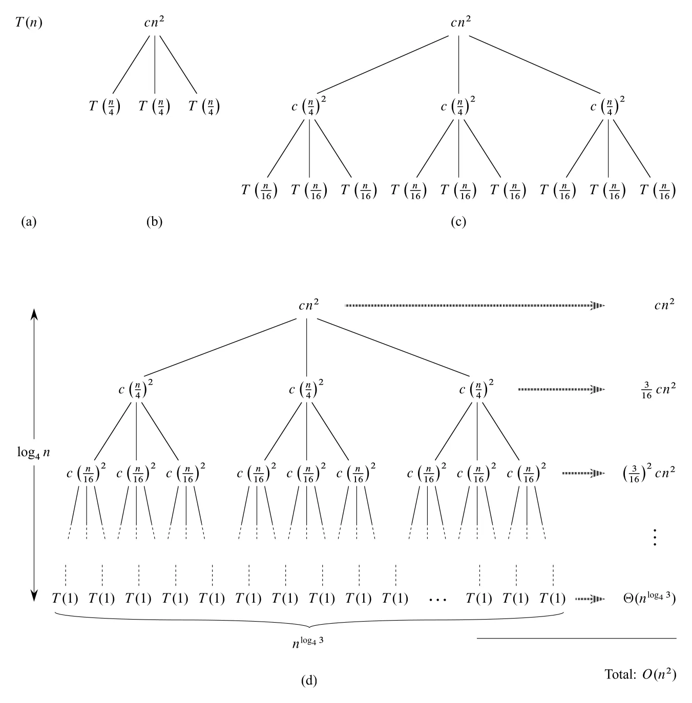Figure 4.5 · PDF p. 110 · $T(n) = 3T(n/4) + cn^{2}$의 recursion tree와 level별 비용 감소

Depth $i$의 subproblem size는 $n/4^{i}$다. $n/4^{i} = 1$이 될 때 $i = \log_{4} n$이므로 tree height는 $\log_4 n$이고, level 수는 $\log_4 n + 1$이다.

Depth $i$의 node 수는 $3^{i}$이고, 각 node cost는 $c(n/4^{i})^{2}$다. 따라서 depth $i$의 total cost는

이다. Bottom level에는 $3^{\log_{4} n} = n^{\log_{4} 3}$ leaves가 있고, 각 leaf cost는 constant이므로 leaf total cost는 $\Theta(n^{\log_{4} 3})$이다.

Internal levels의 cost는 decreasing geometric series다.

따라서 total cost는 $O(n^{2})$이다. Root cost $cn^{2}$가 total cost의 constant fraction을 차지하므로 root dominates the tree라고 볼 수 있다. 또한 첫 recursive expansion 자체에 $\Theta(n^{2})$ cost가 있으므로 lower bound도 $\Omega(n^{2})$이고, 결국 tight bound는 $\Theta(n^{2})$다.

Substitution으로 upper bound를 확인하면 다음과 같다.

예 2: $T(n) = T(n/3) + T(2n/3) + cn$

Figure 4.6은 unequal split recurrence를 보여준다.

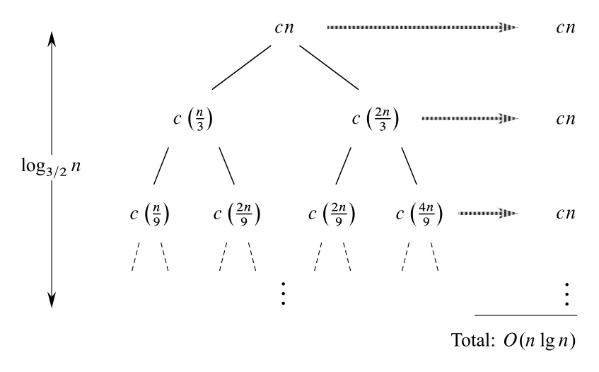Figure 4.6 · PDF p. 112 · $T(n) = T(n/3) + T(2n/3) + cn$의 unequal split recursion tree

상단 levels에서는 각 level의 cost를 합하면 $cn$처럼 보인다. 가장 긴 root-to-leaf path는 매번 $2n/3$ 쪽으로 내려가는 path이고,

이므로 height는 $\log_{3/2} n$이다. 따라서 직관적으로 total cost는 level 수 곱하기 level cost, 즉 $O(n \lg n)$일 것이라고 guess한다.

다만 이 tree는 complete binary tree가 아니다. 아래쪽으로 갈수록 subproblem들이 먼저 leaf에 도달해 internal nodes가 빠지므로, 모든 level이 정확히 $cn$을 기여하지는 않는다. 그래도 upper-bound guess로는 충분하다.

Substitution으로 $T(n) \le d n \lg n$을 검증하면:

마지막 부등식은 $d \ge c / (\lg 3 - 2/3)$이면 성립한다. 따라서 $O(n \lg n)$ upper bound가 검증된다.

Recursion tree를 읽는 순서

Recursion-tree method를 사용할 때는 다음 순서로 보면 좋다.

이 흐름은 Section 4.5의 master theorem 세 cases와도 연결된다. 어떤 경우에는 leaves가 지배하고, 어떤 경우에는 모든 levels가 비슷하게 기여하며, 어떤 경우에는 root 근처의 work가 지배한다.

4.5 The master method for solving recurrences

Master method의 대상

Master method는 다음 꼴의 recurrence를 빠르게 푸는 cookbook method다.

여기서 $a \ge 1$, $b > 1$은 constants이고, $f(n)$은 asymptotically positive function이다. 이 recurrence는 size $n$ 문제를 $a$개의 subproblems로 나누고, 각 subproblem size가 $n/b$이며, divide와 combine의 전체 cost가 $f(n)$인 divide-and-conquer algorithm을 나타낸다.

예를 들어 Strassen’s algorithm은 $a = 7$, $b = 2$, $f(n) = \Theta(n^{2})$이다.

Floors와 ceilings는 보통 생략한다. 실제로는 $T(\lfloor n/b \rfloor)$ 또는 $T(\lceil n/b \rceil)$가 되어야 하지만, master theorem은 이런 rounding이 asymptotic behavior를 바꾸지 않음을 보장한다.

Theorem 4.1: Master theorem

Master theorem은 $f(n)$과 $n^{\log_{b} a}$를 비교한다. 여기서 $n^{\log_{b} a}$는 recursion leaves 또는 recursive subproblem proliferation이 만들어 내는 기준 성장률이다.

Case 3의 추가 조건 $a f(n/b) \le c f(n)$은 regularity condition이다. 이는 $f(n)$이 충분히 규칙적으로 커져서 상위 level의 work가 하위 level들의 total work보다 일정 비율 이상 크다는 뜻이다. 원문은 우리가 만나는 대부분의 polynomially bounded functions에서는 이 조건이 만족된다고 설명한다.

Polynomially smaller/larger 조건

Master theorem의 세 cases는 단순히 $f(n)$이 작다/같다/크다만 보지 않는다.

• Case 1에서는 $f(n)$이 $n^{\log_{b} a}$보다 polynomially smaller해야 한다. 즉 어떤 $\varepsilon > 0$만큼 지수 차이가 있어야 한다.
• Case 3에서는 $f(n)$이 $n^{\log_{b} a}$보다 polynomially larger해야 하며, regularity condition도 만족해야 한다.
• $f(n)$이 더 작거나 크더라도 polynomial factor만큼 차이 나지 않으면 gaps에 빠져 master method를 적용할 수 없다.

대표적인 gap 예시는 다음 recurrence다.

여기서 $a = 2$, $b = 2$, $n^{\log_{b} a} = n$, $f(n) = n \lg n$이다. $f(n)$은 $n$보다 asymptotically larger이지만, ratio가 $\lg n$뿐이라 어떤 $n^\varepsilon$보다도 작다. 따라서 Case 3의 polynomially larger 조건을 만족하지 못하고, master method를 바로 적용할 수 없다.

사용 예시

Master method는 $a$, $b$, $f(n)$을 확인하고 $f(n)$을 $n^{\log_{b} a}$와 비교하면 된다.

Case 3 regularity check 예시는 다음과 같다.

앞선 알고리즘들의 recurrence 풀기

Maximum-subarray divide-and-conquer와 merge sort의 recurrence는 동일하다.

여기서 $a = 2$, $b = 2$, $n^{\log_{b} a} = n$, $f(n) = \Theta(n)$이므로 Case 2다.

Simple divide-and-conquer matrix multiplication은

이고 $a = 8$, $b = 2$, $n^{\log_{2} 8} = n^{3}$이다. $f(n) = \Theta(n^{2})$는 polynomially smaller이므로 Case 1이다.

Strassen’s algorithm은

이고 $a = 7$, $b = 2$, $n^{\log_{2} 7} = n^{\lg 7}$이다. $2.80 < \lg 7 < 2.81$이고 $f(n)=\Theta(n^{2})$는 $n^{\lg 7}$보다 polynomially smaller이므로 Case 1이다.

이 결과가 Strassen이 straightforward $\Theta(n^{3})$ matrix multiplication보다 asymptotically faster한 이유다.

4.6 Proof of the master theorem

이 절은 master theorem을 적용하는 데 필수는 아니지만, 왜 세 case가 생기는지 설명한다. 증명은 두 단계다. 먼저 $n$이 정확히 $b$의 거듭제곱(exact powers of $b$)일 때 recurrence tree를 분석한다. 그다음 실제 알고리즘처럼 $\lfloor n/b \rfloor$, $\lceil n/b \rceil$가 들어가는 모든 양의 정수 $n$으로 확장한다.

주의할 점은 제한된 domain에서의 asymptotic notation이다. 예를 들어 어떤 함수가 $n=1,2,4,8,\ldots$에서만 $O(n)$이어도, 다른 $n$에서 $n^{2}$처럼 정의되어 있다면 전체 domain에서는 $O(n)$이라고 말할 수 없다. 그래서 proof는 exact powers에서 직관을 얻되, 마지막에 floor/ceiling을 따로 처리한다.

4.6.1 The proof for exact powers

대상 recurrence는 다음 master recurrence다.

여기서 $a \ge 1$, $b > 1$, $f(n)$은 nonnegative function이고, 우선 $n = b^{i}$라고 가정한다. Lemma 4.2는 이 recurrence를 직접 푸는 대신, recursion tree의 level cost 합으로 바꾼다.

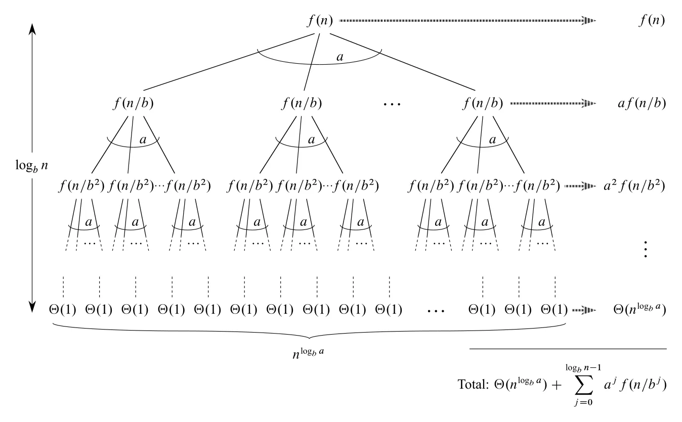Figure 4.7 · PDF p. 120 · $T(n)=aT(n/b)+f(n)$이 만드는 complete a-ary recursion tree

tree에서 depth $j$에는 node가 $a^{j}$개 있고, 각 node의 subproblem size는 $n/b^{j}$다. 따라서 depth $j$의 internal-node cost는

이다. leaf는 $n/b^{j} = 1$이 되는 depth, 즉 $j = \log_{b} n$에 있고, leaf 수는

개다. leaf 하나의 cost는 $\Theta(1)$이므로 leaf 전체 cost는 $\Theta(n^{\log_{b} a})$다. 따라서 exact powers에서 전체 시간은

로 표현된다. 이 식에서 앞 항은 leaves cost, 뒤의 summation은 divide/combine cost의 level별 합이다. master theorem의 세 case는 이 tree에서 비용이 어디에 몰리는지에 대한 분류다.

Lemma 4.3은 summation

을 세 상황에서 평가한다.

Case 1에서는 $f(n)=O(n^{\log_{b} a - \varepsilon})$이다. $f(n/b^{j})$를 대입하면 level cost가 geometric series 형태가 되고, 전체 internal cost는 $O(n^{\log_{b} a})$를 넘지 않는다. leaf cost도 $\Theta(n^{\log_{b} a})$이므로 최종적으로 $T(n)=\Theta(n^{\log_{b} a})$다.

Case 2에서는 $f(n)=\Theta(n^{\log_{b} a})$이다. 이때 각 level의 cost가 모두 같은 차수다.

level이 $\log_b n$개 있으므로 internal cost는 $\Theta(n^{\log_{b} a} \lg n)$이고, leaf cost보다 크거나 같은 차수라서 전체도 $\Theta(n^{\log_{b} a} \lg n)$이다.

Case 3에서는 regularity condition

이 중요하다. 이 조건은 한 level 아래로 내려갈 때 전체 level cost가 적어도 일정 비율로 줄어든다는 뜻이다. 반복하면

가 되어 internal cost가 decreasing geometric series가 된다.

또한 summation의 첫 항이 $f(n)$이므로 $g(n)=\Omega(f(n))$이고, 결국 $g(n)=\Theta(f(n))$이다. 여기에 $f(n)=\Omega(n^{\log_{b} a+\varepsilon})$가 붙으면 leaf cost $\Theta(n^{\log_{b} a})$는 $f(n)$보다 작아서 $T(n)=\Theta(f(n))$가 된다.

4.6.2 Floors and ceilings

실제 recurrence는 보통 subproblem size가 정확히 $n/b$가 아니라 $\lfloor n/b \rfloor$ 또는 $\lceil n/b \rceil$다.

proof는 exact powers에서 얻은 tree가 floor/ceiling 때문에 크게 망가지지 않음을 보인다. ceiling recurrence의 recursive argument를

로 두면, $\lceil x \rceil \le x + 1$이므로 다음 bound를 얻는다.

$j = \lfloor \log_{b} n \rfloor$이면 $n_{j} = O(1)$이므로 tree depth는 여전히 $\Theta(\lg n)$이다. 따라서 ceiling이 있어도 tree는 대략 Figure 4.8처럼 읽을 수 있다.

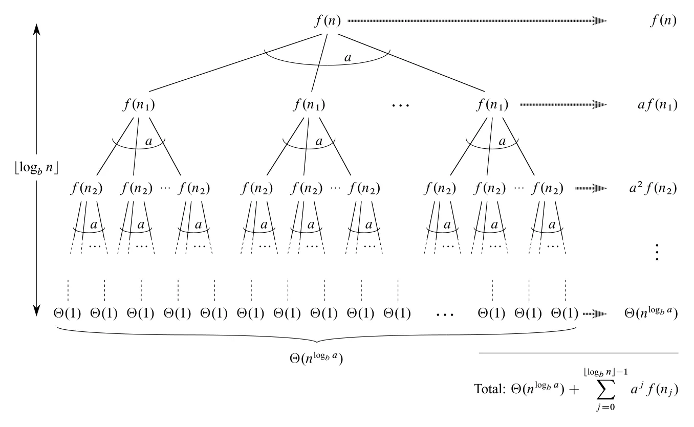Figure 4.8 · PDF p. 125 · $T(n)=aT(\lceil n/b \rceil)+f(n)$에서 recursive argument $n_{j}$를 쓰는 recursion tree

전체 cost는 exact powers의 식과 거의 같은 형태가 된다.

Case 3에서는 regularity condition을 $a f(\lceil n/b \rceil) \le c f(n)$ 형태로 쓰면 $a^{j} f(n_{j}) \le c^{j} f(n)$이 되어 exact powers proof와 같은 decreasing geometric series가 나온다. Case 2에서는 $n_{j} < n/b^{j} + b/(b-1)$를 이용해 $f(n_{j})=O(n^{\log_{b} a}/a^{j})$를 보이면 각 level cost가 $O(n^{\log_{b} a})$로 유지된다. Case 1도 같은 구조지만 지수에 $-\varepsilon$가 들어가 algebra가 조금 더 복잡할 뿐이다.

핵심은 floor/ceiling이 recursion depth와 level cost를 상수배 이상으로 흔들지 않는다는 점이다. 그래서 master theorem은 exact powers뿐 아니라 모든 integer input size에 적용된다.

Proof가 알려주는 사용상의 감각

$n^{\log_{b} a}$는 leaf가 얼마나 많아지는지를 나타낸다. 이것은 “recursive branching이 만들어내는 일의 양”이다. 반대로 $f(n)$은 각 node에서 recursive calls 바깥으로 수행하는 divide/combine cost다. master method는 이 둘의 성장률을 비교해 tree의 어느 부분이 총합을 지배하는지 판단한다.

예를 들어 $T(n)=4T(n/2)+n^{2} \lg n$에서는 $n^{\log_{2} 4}=n^{2}$이고 $f(n)=n^{2} \lg n$이다. $f(n)$은 $n^{2}$보다 크지만 polynomially larger가 아니라 logarithmic factor만 크다. 따라서 기본 master theorem의 Case 3으로 곧장 처리할 수 없다. 이런 경우에는 recursion tree, substitution method, 또는 확장된 master theorem이 필요하다.

Exercises, problems, chapter notes에서 남겨야 할 연결

Chapter 4의 exercises와 problems는 단순 계산 문제가 아니라 이 장의 method들이 어디까지 적용되는지 확인하게 한다.

• $4.5-2$는 Strassen보다 빠른 matrix multiplication을 만들려면 $T(n)=aT(n/4)+\Theta(n^{2})$에서 $a$가 얼마나 작아야 하는지 묻는다. 비교 대상은 $\Theta(n^{\lg 7})$이므로 $n^{\log_{4} a}$와 $n^{\lg 7}$를 비교해야 한다.
• $4.5-4$, $4.6-2$는 $f(n)=n^{\log_{b} a} \lg^{k} n$처럼 boundary case에 logarithmic factor가 붙을 때 기본 master theorem만으로는 부족하다는 점을 보여준다.
• $4.6-3$은 Case 3의 regularity condition이 단순한 부가 조건이 아니라 $f(n)$이 실제로 $n^{\log_{b} a}$보다 polynomially 커지는 성질과 연결된다는 점을 확인하게 한다.
• 4-2 Parameter-passing costs는 알고리즘의 abstract recurrence가 programming model assumption에 의존함을 보여준다. 배열을 pointer로 넘기면 procedure call cost는 $\Theta(1)$이지만, array copying을 하면 recurrence의 $f(n)$이 달라진다.
• 4-3 More recurrence examples에는 $T(n/2)+T(n/4)+T(n/8)+n$처럼 equal-size subproblems가 아닌 recurrence가 나오며, 이는 master method의 적용 범위를 넘어선다.
• 4-4 Fibonacci numbers는 recurrence를 generating functions로 푸는 예고편이다. 모든 recurrence가 divide-and-conquer tree로만 풀리는 것은 아니다.
• 4-5 Chip testing은 divide-and-conquer가 numeric recurrence뿐 아니라 pairwise test로 problem size를 줄이는 identification problem에도 쓰임을 보여준다.
• 4-6 Monge arrays는 구조적 성질(Monge array, row minima의 monotonicity)을 이용해 divide-and-conquer search 범위를 줄이는 예다.

Chapter notes의 실전적 메시지도 중요하다. Strassen’s algorithm은 asymptotically faster이지만 항상 practical winner는 아니다. hidden constant가 크고, sparse matrices에는 특화 알고리즘이 더 빠르며, numerical stability와 extra space 문제가 있다. 실제 dense matrix multiplication 구현은 큰 matrix에서는 Strassen을 쓰다가 subproblem이 crossover point 아래로 작아지면 straightforward method로 바꾸는 hybrid 방식을 쓴다. 이 crossover point는 cache, pipelining, machine architecture에 크게 의존한다.

마지막으로 master method는 간단하지만 equal subproblem size recurrence에 맞춰져 있다. $T(n)=T(\lfloor n/3 \rfloor)+T(\lfloor 2n/3 \rfloor)+O(n)$ 같은 recurrence는 master method로 직접 풀 수 없고, 더 일반적인 Akra-Bazzi method가 필요하다. Akra-Bazzi는 여러 비율의 subproblems를 허용하며, $\sum a_{i} b_{i}^{p} = 1$을 만족하는 p를 찾은 뒤 integral term으로 해를 표현한다.

복잡도

연결 관계

• Chapter 2의 insertion sort, merge sort, loop invariant와 연결된다. 특히 merge sort recurrence $T(n)=2T(n/2)+\Theta(n)$은 Chapter 4에서 recursion tree와 master method로 다시 분석된다.
• Chapter 3의 asymptotic notation, polynomially larger/smaller, $\lg n$, $\Theta$, $O$, $\Omega$ 없이는 master theorem의 조건을 정확히 읽을 수 없다.
• 이 장의 recurrence-solving tools는 이후 sorting, selection, dynamic programming, graph algorithms에서 반복적으로 쓰인다.
• Strassen’s algorithm은 asymptotic analysis와 practical performance가 다를 수 있음을 보여주는 대표 예다. asymptotic improvement가 있어도 constants, memory, numerical stability, sparsity가 실제 선택을 바꾼다.
• Akra-Bazzi method는 master method의 한계를 보완하는 더 일반적인 recurrence 도구로, unequal subproblem sizes를 다룰 때 연결된다.