개요
greedy algorithm은 optimization problem에서 매 단계 “지금 보기에는 가장 좋은 선택”, 즉 locally optimal choice를 한다. 목표는 이 선택들의 누적이 globally optimal solution으로 이어지는 문제들을 찾는 것이다.
Chapter 15의 dynamic programming은 가능한 choices를 비교하기 위해 subproblems를 먼저 풀고 table에 저장했다. Greedy는 반대로 choice를 먼저 한다. 따라서 빠르고 단순할 수 있지만, 모든 문제에서 맞지는 않는다. 이 장의 핵심은 “언제 greedy choice가 안전한가?”를 증명하는 방법이다.
이 장의 흐름은 다음과 같다.
| Section | 핵심 |
|---|---|
16.1 activity-selection problem | DP처럼 보이는 문제에서 earliest finish time greedy choice가 최적인 이유 |
16.2 greedy strategy | greedy-choice property와 optimal substructure를 증명하는 일반 패턴 |
16.3 Huffman codes | data compression의 prefix code를 greedy로 만드는 대표 사례 |
16.4 matroids | greedy가 항상 통하는 조합 구조의 이론 |
16.5 task scheduling | matroid로 unit-time tasks scheduling 문제를 푸는 방법 |
핵심 개념
| 용어 | 뜻 | 검색 키워드 |
|---|---|---|
| greedy algorithm | 각 단계에서 locally best choice를 해 solution을 구성하는 알고리즘 | greedy algorithm |
| greedy-choice property | 어떤 optimal solution이 greedy choice를 포함하도록 항상 바꿀 수 있는 성질 | greedy-choice property |
| optimal substructure | optimal solution이 subproblems의 optimal solutions를 포함하는 성질 | optimal substructure |
| activity-selection problem | 서로 겹치지 않는 activities를 최대 개수로 고르는 scheduling 문제 | activity-selection problem |
| compatible activities | time intervals가 겹치지 않는 activities | compatible |
| earliest finish time | 가장 빨리 끝나는 activity를 먼저 고르는 greedy rule | earliest finish time |
세부 정리
16.1 An activity-selection problem
activity-selection problem은 하나의 common resource를 여러 activities가 독점적으로 쓰고 싶어 할 때, 서로 겹치지 않는 activities를 최대 개수로 고르는 문제다. 예를 들어 lecture hall은 한 번에 한 activity만 진행할 수 있으므로, 가능한 많은 강의/행사를 배정하려면 intervals가 겹치지 않는 subset을 골라야 한다.
Problem definition
활동 집합을 이라 하자. 각 activity 는 start time 와 finish time 를 가지며, 실제 사용 interval은 half-open interval [s_i, f_i)다.
두 activities , 가 compatible하려면 interval이 겹치지 않아야 한다.
입력 activities는 finish time이 nondecreasing order로 정렬되어 있다고 가정한다.
원문 예시는 다음 11개 activities를 사용한다.
| i | 1 | 2 | 3 | 4 | 5 | 6 | 7 | 8 | 9 | 10 | 11 |
|---|---|---|---|---|---|---|---|---|---|---|---|
| 1 | 3 | 0 | 5 | 3 | 5 | 6 | 8 | 8 | 2 | 12 | |
| 4 | 5 | 6 | 7 | 9 | 9 | 10 | 11 | 12 | 14 | 16 |
{a_3, a_9, a_11}은 compatible하지만 maximum-size subset은 아니다. {a_1, a_4, a_8, a_11}과 {a_2, a_4, a_9, a_11}은 크기 4의 maximum-size compatible subsets다.
Dynamic-programming view
Activity-selection은 먼저 DP 문제처럼 볼 수 있다. 를 activity 가 끝난 뒤 시작하고, activity 가 시작하기 전에 끝나는 activities의 집합이라고 하자. 의 optimal solution 가 어떤 activity 를 포함한다면, 문제는 두 subproblems로 갈라진다.
즉 보다 앞에 배치할 compatible activities와 뒤에 배치할 compatible activities를 각각 최적으로 골라야 한다. Cut-and-paste argument로 안의 왼쪽/오른쪽 subsolutions도 optimal이어야 함을 보일 수 있다. 더 좋은 오른쪽 subsolution이 있다면 의 오른쪽 부분만 교체해 전체 activity 수를 늘릴 수 있어 contradiction이다.
를 에서 고를 수 있는 maximum-size compatible subset의 크기라고 하면:
이 recurrence는 matrix-chain multiplication과 비슷하게 가능한 split/activity 를 모두 시도하게 만든다. Memoized recursion이나 bottom-up table로 풀 수 있지만, 이 문제에는 더 강한 성질이 있다.
Greedy choice: earliest finish time
Greedy intuition은 “resource를 가능한 빨리 비워서 뒤의 activities가 들어올 여지를 많이 남기자”이다. 따라서 현재 남은 activities 중 finish time이 가장 이른 activity를 고른다. 입력이 finish time 순서로 정렬되어 있으면 처음 선택은 이다.
을 선택하면 왜 왼쪽 subproblem이 없어지는가? 은 전체에서 가장 이른 finish time이고 이다. 따라서 어떤 activity도 이전 또는 까지 끝날 수 없다. 결국 과 compatible한 activities는 모두 이 끝난 뒤 시작하는 activities뿐이다.
를 activity 가 끝난 뒤 시작하는 activities의 subproblem이라고 하자. Greedy가 을 고르면 남는 문제는 하나뿐이다. 이 점이 DP의 “두 subproblems를 모두 풀고 choice를 고르는 방식”과 다르다.
Theorem 16.1: greedy choice is safe
Theorem 16.1은 activity-selection problem에서 earliest finish time choice가 어떤 optimal solution에 포함됨을 보인다.
임의의 nonempty subproblem 에서 finish time이 가장 이른 activity를 이라 하면, 은 의 maximum-size mutually compatible subset 중 적어도 하나에 포함된다.
증명은 exchange argument다.
- 를 의 maximum-size compatible subset이라고 하자.
- 안에서 가장 먼저 끝나는 activity를 라고 하자.
- 만약 이면 이미 greedy choice가 optimal solution 안에 있다.
- 아니라면 으로 바꾼다.
- 은 에서 가장 빨리 끝나므로 다. 에서 뒤에 오던 activities는 와 compatible했으므로, 더 일찍 끝나는 과도 compatible하다.
- 따라서
A'_k도 compatible하고 크기는 와 같다. 즉 을 포함하는 maximum-size solution이 존재한다.
이 증명은 greedy correctness에서 자주 쓰이는 형태다. 어떤 optimal solution이 greedy choice를 포함하지 않더라도, 첫 선택을 greedy choice로 “교환(exchange)”해도 optimality가 깨지지 않음을 보인다.
Recursive greedy algorithm
RECURSIVE-ACTIVITY-SELECTOR는 fictitious activity 을 추가해 시작한다. 이고, initial call은 RECURSIVE-ACTIVITY-SELECTOR(s, f, 0, n)이다. 가 전체 activity set이 된다.
RECURSIVE-ACTIVITY-SELECTOR(s, f, k, n)
1  m = k + 1
2  while m <= n and s[m] < f[k]
3      m = m + 1
4  if m <= n
5      return {a_m} ∪ RECURSIVE-ACTIVITY-SELECTOR(s, f, m, n)
6  else return ∅
Line 2-3은 현재 선택된 마지막 activity 와 compatible한 첫 activity 을 찾는다. Activities가 finish time 순서로 정렬되어 있으므로, 이 은 에서 가장 빨리 끝나는 activity다. 찾으면 을 선택하고 subproblem 을 재귀적으로 푼다. 더 이상 compatible activity가 없으면 empty set을 반환한다.
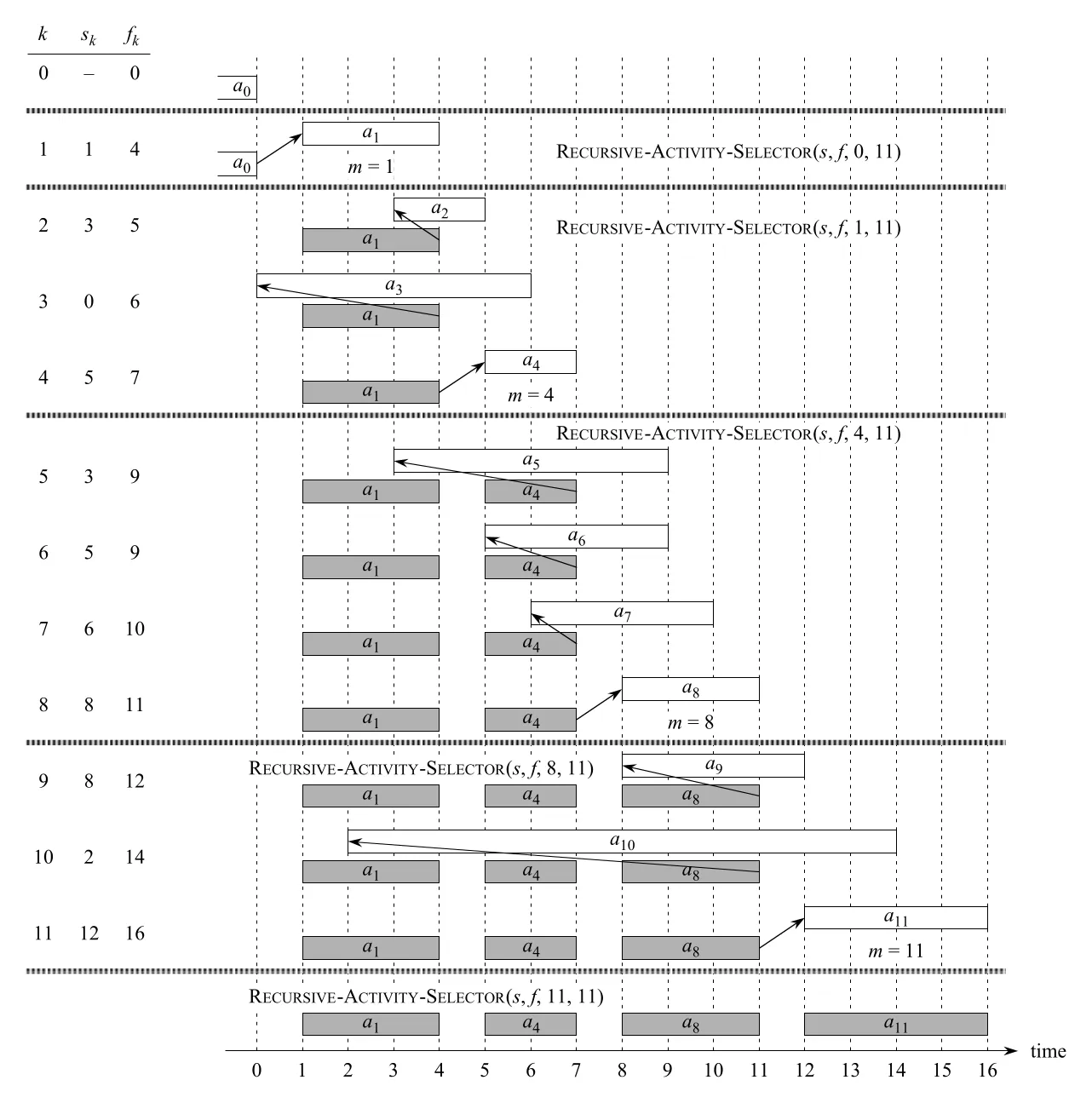 Figure 16.1 · PDF p. 441 ·
 RECURSIVE-ACTIVITY-SELECTOR가 activities를 순서대로 선택/거절하는 과정
Figure 16.1은 원문 11개 activities에서 recursive calls가 , , , 을 선택하는 과정을 보여 준다. Shaded activities는 이미 선택된 것들이고, white activity는 현재 검사 중인 activity다. Start time이 최근 선택 activity의 finish time보다 작으면 거절하고, 그렇지 않으면 선택한다.
정렬이 이미 되어 있다면 running time은 이다. 모든 recursive calls 전체에서 각 activity는 while loop test에서 정확히 한 번씩 검사된다. 정렬이 필요하면 finish time 기준 sorting 때문에 전체 시간은 이 된다.
Iterative greedy algorithm
Recursive version은 거의 tail recursive이므로 iterative form으로 쉽게 바뀐다. GREEDY-ACTIVITY-SELECTOR는 선택된 activities를 set A에 모으고, k를 가장 최근에 선택한 activity index로 유지한다.
GREEDY-ACTIVITY-SELECTOR(s, f)
1  n = s.length
2  A = {a_1}
3  k = 1
4  for m = 2 to n
5      if s[m] >= f[k]
6          A = A ∪ {a_m}
7          k = m
8  return A
입력이 finish time 순서로 정렬되어 있으므로, loop가 어떤 compatible activity를 처음 발견하는 순간 그것이 현재 subproblem에서 earliest finish time activity다. Compatibility는 모든 기존 selected activities와 비교할 필요가 없다. 선택된 activities의 finish times는 증가하고, k가 가장 최근 선택 activity이자 현재 A 안에서 finish time이 가장 큰 activity를 가리키기 때문이다.
따라서 새 activity 이 전체 A와 compatible한지 확인하려면 만 검사하면 된다. Iterative algorithm도 sorting 후에는 time이다.
Greedy가 실패하는 변형들
Activity-selection에서 “빨리 끝나는 activity”는 안전하지만, 아무 greedy rule이나 되는 것은 아니다. 원문 exercises는 다음 rules가 실패할 수 있음을 묻는다.
| Greedy rule | 왜 위험한가 |
|---|---|
| duration이 가장 짧은 activity 선택 | 짧아도 중앙에 끼어 양쪽의 많은 compatible activities를 막을 수 있음 |
| 남은 activities와 overlap이 가장 적은 activity 선택 | local overlap 수가 전체 chain 구조의 최적성을 보장하지 않음 |
| earliest start time 선택 | 너무 길게 이어지는 activity를 먼저 잡아 뒤의 many activities를 막을 수 있음 |
또한 activity마다 value 가 붙어 “개수 최대화”가 아니라 “총 value 최대화”가 목표가 되면 earliest finish time greedy가 충분하지 않다. 이 변형은 weighted interval scheduling 형태로 polynomial-time DP가 필요하다.
16.2 Elements of the greedy strategy
Greedy algorithm은 sequence of choices로 optimal solution을 만든다. 매 decision point에서 현재 가장 좋아 보이는 choice를 고르지만, 이 heuristic이 항상 맞지는 않는다. Greedy가 맞는 문제에서는 보통 두 성질을 증명한다.
greedy-choice property: locally optimal choice를 포함하는 globally optimal solution이 항상 존재한다.optimal substructure: greedy choice를 한 뒤 남는 subproblem의 optimal solution과 greedy choice를 결합하면 원래 문제의 optimal solution이 된다.
From dynamic programming to greedy
16.1의 activity-selection problem은 greedy를 설계하는 과정을 DP 기반으로 보여 주었다.
| 단계 | 16.1에서 한 일 |
|---|---|
| 1 | 로 optimal substructure를 찾음 |
| 2 | recurrence (16.2)로 recursive DP 형태를 세움 |
| 3 | greedy choice를 하면 subproblem이 하나만 남음을 관찰 |
| 4 | earliest finish time choice가 safe함을 Theorem 16.1로 증명 |
| 5 | recursive greedy algorithm 작성 |
| 6 | iterative greedy algorithm으로 변환 |
하지만 실제 greedy 설계는 더 직접적으로 할 수 있다. 처음부터 “choice 하나를 하면 subproblem 하나만 남는” formulation을 잡고, 그 choice가 안전함을 증명한다. Activity-selection에서는 대신 를 subproblem으로 보고, 에서 가장 빨리 끝나는 activity 을 고른 뒤 남은 을 푸는 식으로 바로 접근할 수 있다.
Greedy 아래에는 대개 더 무거운 dynamic-programming solution이 숨어 있다. Greedy는 그중 일부 choices만 고려해도 충분하다는 증명이 있을 때 DP를 단순화한다.
Greedy-choice property
greedy-choice property는 현재 문제에서 locally best choice를 먼저 해도 global optimality를 잃지 않는다는 성질이다. Dynamic programming과의 차이는 choice의 시점이다.
| 전략 | Choice를 언제 하나? | Subproblems와의 관계 |
|---|---|---|
| dynamic programming | subproblems를 풀고 난 뒤 선택 | choice가 subproblem solutions에 의존 |
| top-down memoized DP | 코드 흐름은 top-down이어도 choice 전에 필요한 subproblems를 계산 | cache로 중복 제거 |
| greedy algorithm | subproblems를 풀기 전에 먼저 선택 | choice가 future choices나 subproblem solutions에 의존하면 안 됨 |
Greedy proof는 보통 exchange argument 형태다. 어떤 subproblem의 globally optimal solution을 잡고, 그 안의 첫 choice를 greedy choice로 바꿔도 solution quality가 나빠지지 않음을 보인다. 그러면 greedy choice를 포함하는 optimal solution이 존재한다.
Greedy choice는 보통 preprocessing이나 data structure로 빠르게 만들 수 있다. Activity-selection에서는 finish time sorting 후 한 번 scan하면 됐다. 다른 문제에서는 priority queue가 greedy choice를 빠르게 꺼내는 대표 도구다.
Optimal substructure in greedy
Greedy에서도 optimal substructure가 필요하다. 다만 DP에서처럼 모든 candidate choices를 열거하고 recurrence를 세우기보다, greedy choice를 이미 했다고 가정한 뒤 남은 subproblem이 최적이어야 함을 보인다.
즉 증명 목표는 다음 형태다.
이 논리는 보통 induction으로 확장된다. 첫 greedy choice가 안전하고, 남은 subproblem도 같은 구조를 가진다면, 같은 논리를 반복해 전체 greedy sequence가 optimal solution을 만든다.
Greedy versus dynamic programming: knapsack
Greedy와 DP의 차이를 보여 주는 대표 예가 knapsack problem이다.
0-1 knapsack problem에서는 각 item i가 value , weight 를 가지며, thief는 capacity W 이하에서 value 합을 최대화하고 싶다. 각 item은 take 또는 leave만 가능하다. 즉 fraction을 가져갈 수 없다.
fractional knapsack problem은 같은 설정이지만 item을 쪼개서 가져갈 수 있다. Gold ingot은 0-1 knapsack에 가깝고, gold dust는 fractional knapsack에 가깝다.
두 문제 모두 optimal substructure는 있다.
| 문제 | Optimal substructure |
|---|---|
| 0-1 knapsack | optimal load에서 item j를 제거하면, 남은 load는 capacity 와 item j 제외 조건에서 optimal이어야 함 |
| fractional knapsack | item j의 weight w만큼 제거하면, 남은 load는 capacity W-w에서 optimal이어야 함 |
하지만 greedy-choice property는 fractional knapsack에만 성립한다. Fractional knapsack에서는 value density v_i / w_i가 가장 큰 item부터 가능한 만큼 담으면 된다. 한 item이 다 떨어져도 capacity가 남으면 다음 density item을 담는다. Sorting을 쓰면 time이다.
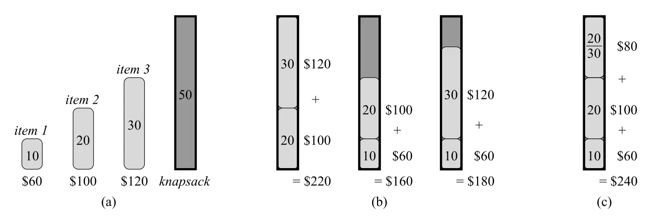 Figure 16.2 · PDF p. 448 ·
 0-1 knapsack에서는 value density greedy가 실패하지만 fractional에서는 성공하는 예
Figure 16.2의 instance는 capacity 50이고 items는 다음과 같다.
| item | weight | value | value per pound |
|---|---|---|---|
| 1 | 10 | 60 | 6 |
| 2 | 20 | 100 | 5 |
| 3 | 30 | 120 | 4 |
Value density greedy는 item 1을 먼저 고른다. 하지만 0-1 knapsack의 optimal solution은 item 2와 item 3을 담아 total value 220을 얻는 것이다. Item 1을 포함하는 가능한 선택들은 160 또는 180에 그쳐 suboptimal이다.
반대로 fractional knapsack에서는 item 1, item 2를 모두 담고 item 3의 일부를 담아 total value 240을 얻는다. Fraction을 허용하면 capacity를 value density 순서대로 꽉 채울 수 있으므로 greedy가 맞는다.
왜 0-1 knapsack은 DP가 필요한가
0-1 knapsack에서 어떤 item을 넣을지 말지는 나중의 조합 가능성을 바꾼다. Item 1의 density가 높아도, 그것을 넣으면 남는 capacity가 애매해져 전체 value가 낮아질 수 있다. 따라서 item을 포함하는 subproblem과 제외하는 subproblem을 비교해야 한다.
이 비교는 future subproblem solutions에 의존하므로 greedy choice가 아니다. 게다가 같은 (i, W) subproblems가 반복되므로 overlapping subproblems가 생긴다. 그래서 0-1 knapsack은 dynamic programming solution이 자연스럽다.
16.3 Huffman codes
Huffman codes는 characters의 frequencies를 이용해 file을 압축하는 optimal prefix code를 만드는 greedy algorithm이다. 자주 나오는 character에는 짧은 codeword를, 드물게 나오는 character에는 긴 codeword를 배정해 전체 bit 수를 줄인다.
Character coding problem
100,000-character file에 characters a-f만 등장하고 frequencies가 다음과 같다고 하자.
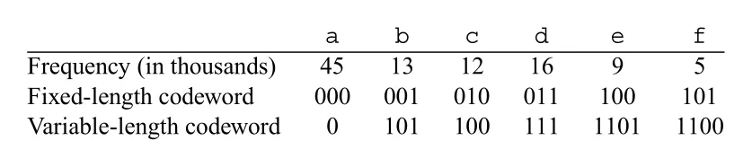 Figure 16.3 · PDF p. 450 · fixed-length code와 variable-length code의 bit 수 비교
6개 characters를 fixed-length code로 표현하려면 character마다 3 bits가 필요하므로 전체 300,000 bits가 든다. 반면 Figure 16.3의 variable-length code는 a를 0, f를 1100처럼 표현해 전체 bit 수를 줄인다.
이 예시는 약 25% saving을 만든다. CLRS는 이 code가 해당 frequencies에 대해 optimal임을 Huffman algorithm으로 보인다.
Prefix codes
prefix code는 어떤 codeword도 다른 codeword의 prefix가 되지 않는 code다. 예를 들어 이라면 0...으로 시작하는 다른 codeword가 없어야 한다. 이 조건은 decoding을 unambiguous하게 만든다.
Encoding은 codewords를 이어 붙이는 것이다. Figure 16.3의 variable-length prefix code에서 abc는 다음처럼 encode된다.
Decoding은 왼쪽부터 codeword 하나씩 끊어 읽는다. Prefix-free 성질 때문에 처음 codeword가 어디서 끝나는지 모호하지 않다. 예를 들어 001011101은 0 · 0 · 101 · 1101로 유일하게 parse되어 aabe가 된다.
Prefix code는 binary tree로 표현하기 좋다. Root에서 왼쪽 edge는 0, 오른쪽 edge는 1로 보고, character leaf까지의 simple path가 codeword가 된다.
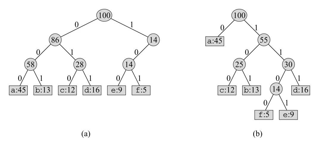 Figure 16.4 · PDF p. 451 · fixed-length code tree와 optimal prefix code tree
Figure 16.4의 tree들은 binary search tree가 아니다. Characters는 leaves에 있고, internal nodes는 keys가 아니라 subtree frequencies sum을 담는다. Optimal prefix code는 항상 full binary tree로 나타낼 수 있다. 즉 모든 internal node가 정확히 두 children을 가진다. Positive frequencies를 가진 alphabet C에 대해 optimal prefix-code tree는 |C| leaves와 |C|-1 internal nodes를 가진다.
Tree T가 prefix code를 나타낼 때, character c의 frequency를 c.freq, leaf depth를 라고 하자. Codeword length가 leaf depth이므로 file encoding bit 수, 즉 tree cost는:
따라서 Huffman coding 문제는 weighted external path length 를 최소화하는 full binary tree를 찾는 문제다.
Huffman algorithm
는 bottom-up으로 optimal prefix-code tree를 만든다. 처음에는 각 character가 leaf node 하나이고, 매 step마다 frequency가 가장 작은 두 nodes를 꺼내 새 internal node의 children으로 merge한다. 새 node의 frequency는 두 frequencies의 합이다.
HUFFMAN(C)
1  n = |C|
2  Q = C
3  for i = 1 to n-1
4      allocate a new node z
5      z.left = x = EXTRACT-MIN(Q)
6      z.right = y = EXTRACT-MIN(Q)
7      z.freq = x.freq + y.freq
8      INSERT(Q, z)
9 return EXTRACT-MIN(Q)Q는 freq를 key로 하는 min-priority queue다. Line 5-6의 두 번의 EXTRACT-MIN이 greedy choice다. 가장 낮은 frequencies의 두 objects를 하나의 subtree로 합치고, 그 subtree를 다시 queue에 넣는다. 번 merge하면 queue에는 root 하나만 남는다.
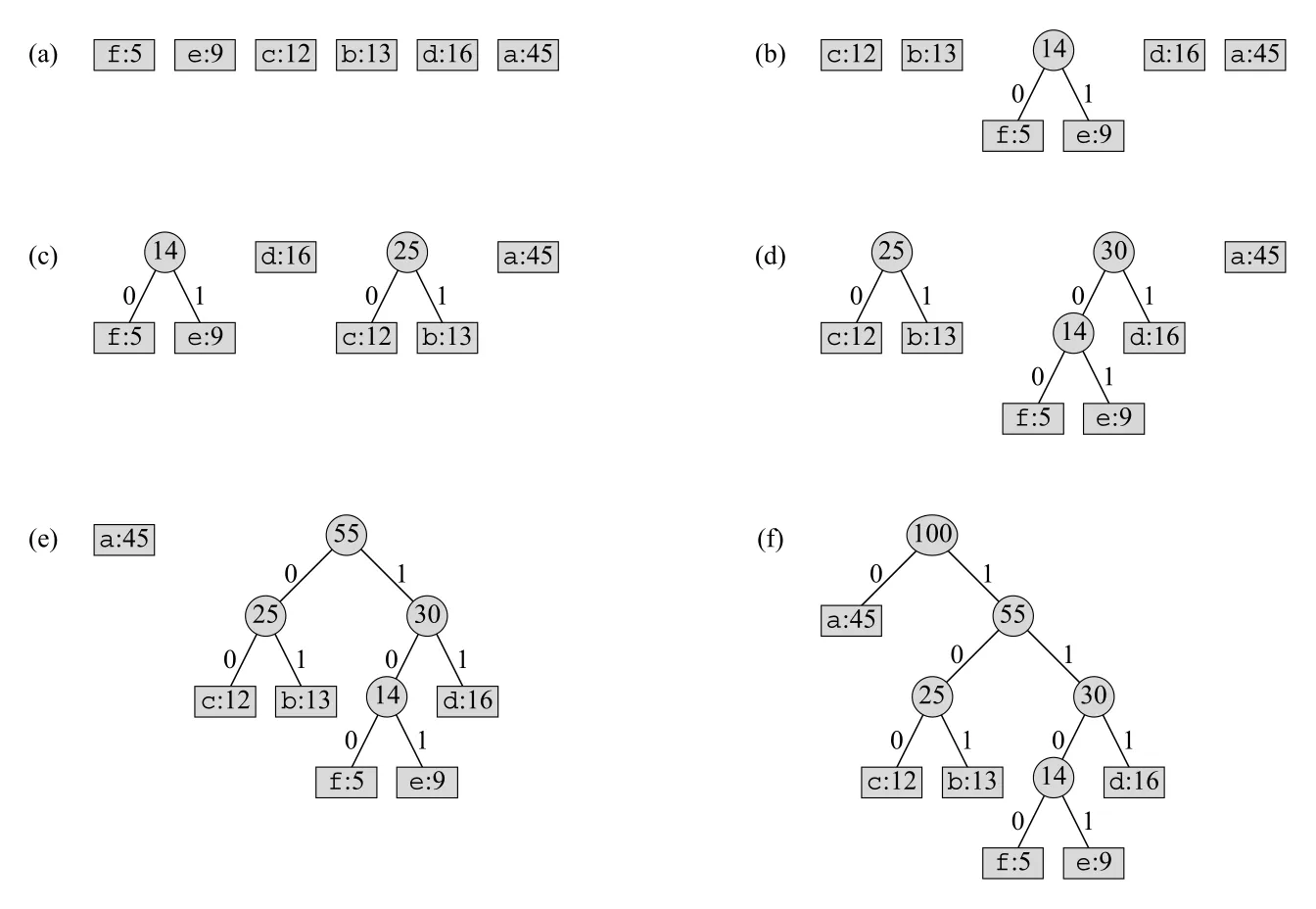 Figure 16.5 · PDF p. 453 · Huffman algorithm이 lowest-frequency trees를 반복 merge하는 과정
Figure 16.5에서는 f:5와 e:9를 먼저 merge해 frequency 14 node를 만든다. 이후 queue에서 항상 가장 작은 두 trees를 merge한다. 최종 tree의 root-to-leaf edge labels가 codewords가 된다. Left/right child 순서는 임의이며, 바꾸면 codeword bit pattern은 달라지지만 cost는 같다.
Binary min-heap을 쓰면 initialization은 BUILD-MIN-HEAP으로 , loop는 번 반복되고 각 반복마다 heap operation이 이므로 total running time은 이다.
Greedy-choice property: Lemma 16.2
Lemma 16.2는 Huffman의 greedy choice가 안전함을 보인다.
Alphabet
C에서 minimum frequencies를 가진 두 characters를x,y라고 하자. 그러면x,y의 codewords가 같은 length이고 마지막 bit만 다른 optimal prefix code가 존재한다.
Tree 관점으로 말하면, minimum-frequency characters x, y를 maximum depth의 sibling leaves로 두는 optimal tree가 존재한다.
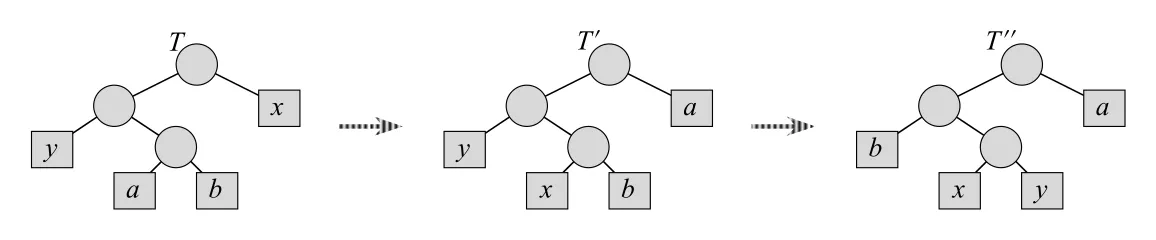 Figure 16.6 · PDF p. 455 · minimum-frequency leaves를 deepest siblings로 교환하는 Lemma 16.2의 핵심
증명 아이디어는 exchange argument다.
- 임의의 optimal tree
T를 잡는다. T에서 maximum depth의 sibling leaves를a,b라고 하자.x,y는 전체에서 frequencies가 가장 작으므로 , 다.a와x의 위치를 swap해T'를 만들고,b와y의 위치를 swap해T''를 만든다.- 낮은 frequency item을 더 깊은 곳에 두는 것은 cost를 증가시키지 않는다.
첫 swap의 cost 차이는 다음처럼 계산된다.
이고 a가 maximum depth leaf라 이기 때문이다. 두 번째 swap도 마찬가지다. 따라서 이고, T가 optimal이므로 T''도 optimal이다. 이제 x, y는 deepest sibling leaves다.
Huffman의 첫 merge는 바로 이 x, y를 siblings로 묶는 선택이다. 가능한 merge들 중 frequency sum이 가장 작으므로 local merge cost도 가장 작다.
Optimal substructure: Lemma 16.3
Lemma 16.3은 Huffman problem의 optimal substructure를 보인다.
Minimum-frequency characters x, y를 하나의 새 character z로 합친 reduced alphabet을 생각하자.
C'에 대한 optimal prefix-code tree T'가 있으면, z leaf를 internal node로 바꾸고 그 children으로 x, y를 붙인 tree T는 원래 alphabet C에 대한 optimal tree다.
Cost 관계는 다음과 같다.
왜냐하면 x, y는 z보다 depth가 1씩 깊어지고, 다른 characters의 depth는 그대로이기 때문이다.
만약 이렇게 만든 T가 optimal이 아니라면, 더 좋은 tree T''가 존재한다. Lemma 16.2에 의해 T''도 x, y를 sibling leaves로 갖도록 바꿀 수 있다. 그 sibling parent를 다시 z leaf로 압축하면 C'에 대한 tree가 되고, 그 cost는 T'보다 작아진다. 이는 T'가 C'에서 optimal이라는 가정과 모순이다.
따라서 “두 minimum-frequency characters를 merge하고 reduced problem을 푼 뒤 다시 펼친다”는 구조가 정당화된다. Theorem 16.4는 Lemma 16.2와 Lemma 16.3으로부터 HUFFMAN이 optimal prefix code를 만든다고 결론낸다.
Huffman coding에서 헷갈리기 쉬운 점
| 항목 | 정리 |
|---|---|
| Prefix code vs fixed-length code | fixed-length code도 prefix code지만, frequencies가 불균등하면 variable-length prefix code가 더 좋다. |
| Code tree vs binary search tree | Huffman tree는 BST가 아니다. Characters는 leaves에 있고 sorted order가 중요하지 않다. |
| Greedy가 고르는 것 | character 자체가 아니라 현재 forest에서 frequency가 가장 작은 두 trees/nodes를 merge한다. |
| Left/right child | 0/1 배정은 arbitrary다. 바꿔도 code cost는 같다. |
| Optimality 증명 | “가장 작은 두 frequencies는 deepest sibling leaves로 둘 수 있다”와 “merge한 reduced problem이 optimal substructure를 가진다”가 핵심이다. |
16.4 Matroids and greedy methods
matroid는 greedy method가 항상 optimal solution을 주는 조합 구조를 추상화한 것이다. 이 이론은 activity-selection이나 Huffman coding까지 모두 포괄하지는 않지만, minimum-spanning-tree 같은 많은 실전 greedy algorithms의 공통 기반을 설명한다.
Matroid definition
Matroid는 ordered pair 다. 여기서 는 finite set이고, 는 의 subsets 중 independent subsets라고 부르는 nonempty family다. 이 matroid가 되려면 다음을 만족해야 한다.
| 조건 | 이름 | 의미 |
|---|---|---|
| is finite | finite ground set | 선택 후보가 유한하다. |
| and 이면 | hereditary property | independent set에서 원소를 제거해도 independent다. Empty set 도 반드시 independent다. |
| 이고 $ | A | < |
hereditary property는 “가능한 선택 집합의 부분집합도 가능하다”는 뜻이고, exchange property는 “큰 feasible solution의 원소 중 하나를 작은 feasible solution에 붙일 여지가 있다”는 뜻이다. Greedy proof에서 이 exchange property가 핵심 역할을 한다.
Graphic matroid
대표 예시는 graphic matroid다. Undirected graph 가 있을 때:
즉 independent subsets는 cycle을 만들지 않는 edge sets다. Subgraph 가 forest이면 는 independent다.
Theorem 16.5는 가 matroid임을 보인다.
| Matroid 조건 | Graphic matroid에서의 이유 |
|---|---|
| finite | edge set 가 finite |
| hereditary | forest에서 edges를 제거해도 cycle이 생기지 않음 |
| exchange | 더 많은 edges를 가진 forest는 더 적은 trees를 가지므로, 큰 forest의 어떤 edge가 작은 forest의 서로 다른 trees를 연결해 cycle 없이 추가될 수 있음 |
Forest 가 개의 trees로 이루어져 있으면:
따라서 이면 forest 는 보다 trees 수가 적다. 그러면 의 어떤 tree 안에는 에서 서로 다른 trees에 속한 두 vertices가 있고, 그 둘을 잇는 edge를 에 추가해도 cycle이 생기지 않는다. 이것이 exchange property다.
Connected undirected graph에서 graphic matroid의 maximal independent subsets는 모두 edges를 가진 spanning trees다.
Extension and maximal independent sets
Matroid 에서 independent set A에 원소 x를 추가해도 independent라면, x를 A의 extension이라고 한다.
Independent set A가 더 이상 extension을 갖지 않으면 maximal independent subset이다. Theorem 16.6은 matroid의 모든 maximal independent subsets가 같은 size를 가진다고 말한다. 만약 maximal independent set A보다 더 큰 maximal independent set B가 있다면, exchange property에 의해 B-A의 어떤 원소를 A에 추가할 수 있어 A의 maximality와 모순이 된다.
이 성질은 “greedy가 원소를 계속 추가해 maximal에 도달했을 때 크기 면에서는 뒤처지지 않는다”는 감각을 준다. 여기에 weights가 들어가면 “어떤 원소를 먼저 추가해야 maximum weight가 되는가?”가 문제다.
Weighted matroid
weighted matroid는 각 element x in S에 positive weight 가 주어진 matroid다. Subset의 weight는 합으로 확장한다.
목표는 maximum-weight independent subset을 찾는 것이다. 모든 weights가 positive이므로 optimal subset은 항상 maximal independent subset이다. 추가 가능한 원소가 남아 있다면 weight가 양수라 더하는 편이 항상 이득이기 때문이다.
Minimum-spanning-tree problem도 matroid 관점으로 볼 수 있다. 원래 MST는 edge length 합을 minimize한다. Matroid greedy theorem은 maximum-weight independent subset을 찾는 형태이므로, 각 edge의 matroid weight를 다음처럼 바꾼다.
여기서 는 모든 edge length보다 큰 상수다. Connected graph의 spanning tree는 항상 |V|-1 edges를 가지므로:
따라서 w'(A)를 maximize하는 것은 원래 length sum 를 minimize하는 것과 같다.
Greedy algorithm on a weighted matroid
Weighted matroid에서 greedy algorithm은 weight가 큰 원소부터 보면서, 추가해도 independent가 유지되면 즉시 추가한다.
GREEDY(M, w)
1  A = ∅
2  sort M.S into monotonically decreasing order by weight w
3  for each x in M.S, taken in monotonically decreasing order by weight w(x)
4      if A ∪ {x} in M.I
5          A = A ∪ {x}
6  return A
Line 4의 independence check가 problem-specific이다. Graphic matroid라면 “edge를 추가했을 때 cycle이 생기는가?”를 검사한다. 이고 independence check가 이면 total time은 sorting plus checks 다.
Correctness of matroid greedy
Matroid greedy correctness는 세 단계로 구성된다.
| 결과 | 의미 |
|---|---|
| Lemma 16.7 | weighted matroid는 greedy-choice property를 가진다. |
| Lemma 16.8 / Corollary 16.9 | 처음에 ∅의 extension이 아닌 원소는 나중에도 어떤 independent set의 extension이 될 수 없다. |
| Lemma 16.10 | greedy choice x를 고른 뒤의 remaining problem은 contraction matroid M'에서 같은 형태의 문제다. |
Lemma 16.7은 weight descending order에서 처음으로 singleton {x}가 independent인 원소 x를 포함하는 optimal subset이 존재함을 보인다. 어떤 optimal subset B가 x를 포함하지 않는다면, hereditary property 때문에 B의 각 원소 y는 singleton {y}가 independent다. x가 가장 먼저 가능한 원소였으므로 다. Exchange property를 이용해 B에서 어떤 y를 빼고 x를 넣어도 independent와 total weight를 유지하거나 높일 수 있다.
Lemma 16.8은 x가 어떤 independent set A의 extension이면 {x} 자체도 independent라고 말한다. 이유는 가 independent이고 hereditary property가 있으므로 그 subset {x}도 independent이기 때문이다. 따라서 contrapositive인 Corollary 16.9에 의해 {x}가 independent가 아니면 x는 어떤 independent set에도 나중에 추가될 수 없다. Greedy가 처음에 skip한 “사용 불가능한” 원소는 영원히 사용 불가능하다.
Lemma 16.10은 greedy가 첫 원소 x를 선택한 뒤 남은 문제가 contraction으로 표현되는 matroid problem임을 보인다.
M' = (S', I')에서 maximum-weight independent subset A'를 찾으면, 원래 matroid에서는 가 x를 포함하는 maximum-weight independent subset이다. Weight 관계는 항상:
Theorem 16.11은 이 세 결과로부터 GREEDY(M, w)가 optimal subset을 반환한다고 결론낸다. Greedy가 처음에 skip한 원소들은 불가능한 원소라 버려도 되고, 처음 선택한 x는 어떤 optimal solution에 포함될 수 있으며, 남은 문제는 contraction matroid에서 동일한 greedy problem이 된다. 이 구조를 반복하면 전체 greedy sequence가 optimal이다.
16.5 A task-scheduling problem as a matroid
이 section은 unit-time tasks를 single processor에서 scheduling하는 문제를 matroid로 바꾸어 greedy algorithm으로 푼다. 문제는 “deadline을 놓친 tasks의 penalty 합을 최소화”하는 것이다.
Problem definition
각 task 는 정확히 one unit of time이 걸린다. Schedule은 tasks의 permutation이다. 첫 task는 time 0에 시작해 1에 끝나고, 두 번째 task는 1에 시작해 2에 끝나는 식이다.
입력은 다음과 같다.
| 입력 | 의미 |
|---|---|
| unit-time tasks | |
| task 의 deadline, | |
| 가 deadline을 놓치면 내는 penalty |
Task가 deadline까지 끝나면 early, deadline 이후에 끝나면 late다. 목표는 late tasks의 penalties 합을 최소화하는 schedule을 찾는 것이다.
Canonical form
임의의 schedule은 optimality를 잃지 않고 다음 형태로 바꿀 수 있다.
- 모든 early tasks가 late tasks보다 앞에 온다.
- Early tasks는 deadline이 nondecreasing order가 되도록 배치된다.
- Late tasks는 뒤에 오며 순서는 penalty에 영향을 주지 않는다.
왜 early-first로 바꿀 수 있는가? 어떤 early task 가 late task 뒤에 있다면 둘을 swap해도 는 더 빨라지므로 early이고, 는 더 늦거나 같은 late 영역에 남으므로 late다.
왜 early tasks를 deadline order로 정렬할 수 있는가? 인접한 두 early tasks , 가 times , 에 끝나는데 라면, 가 이미 early였으므로 다. 둘을 swap해도 는 time 에 끝나 still early이고, 는 time 에 끝나 더 early가 된다.
따라서 실제 scheduling 문제는 “어떤 tasks를 early set 로 둘 것인가?”로 줄어든다. 를 결정하면 를 deadline order로 놓고, 는 뒤에 아무 순서로 두면 된다.
Independent task sets
Task set 가 어떤 schedule에서 모두 early가 될 수 있으면 를 independent라고 한다. 를 모든 independent task sets의 family라고 하자.
를 안에서 deadline이 이하인 tasks 수라고 하자. 이다.
Lemma 16.12는 다음 세 조건이 동치임을 말한다.
| 조건 | 의미 |
|---|---|
| is independent | 의 모든 tasks를 late 없이 schedule할 수 있음 |
| 모든 에 대해 | deadline 까지 끝내야 하는 tasks 수가 available slots 개를 넘지 않음 |
| 를 deadline 증가 순서로 schedule하면 no task is late | EDF(earliest deadline first) 순서가 feasible schedule을 제공 |
핵심은 condition 2다. Deadline이 이하인 tasks가 개를 넘으면, time 전까지 끝내야 하는 tasks가 너무 많으므로 어떤 schedule도 feasible하지 않다. 반대로 이 조건이 모든 에서 성립하면 deadline order로 배치했을 때 막히지 않는다.
Transforming objective
Late penalty를 minimize하는 것은 early tasks의 penalty sum을 maximize하는 것과 같다.
전체 penalty 합은 고정되어 있으므로, late penalty minimization은 independent early set 의 weight maximization으로 바뀐다.
Task sets form a matroid
Theorem 16.13은 와 independent task sets 가 matroid를 이룬다고 말한다.
Hereditary property는 쉽다. 어떤 task set 를 모두 early로 schedule할 수 있다면, 그 subset도 당연히 모두 early로 schedule할 수 있다.
Exchange property는 Lemma 16.12의 조건으로 증명한다. Independent sets , 가 있고 라고 하자. 어떤 deadline level 에서 가 보다 더 많은 tasks를 가지는 첫 구간을 잡을 수 있다. 그러면 deadline이 인 task 를 골라 를 만든다. 에서는 이고, 에서는 라서 도 independent다. 따라서 exchange property가 성립한다.
이제 16.4의 matroid greedy theorem을 그대로 적용할 수 있다. Penalty 를 weight로 보고, 높은 penalty task부터 보면서 early set에 넣어도 independent이면 넣는다. 이렇게 얻은 independent set 가 maximum penalty-sum early set이다.
Greedy scheduling algorithm
Matroid GREEDY를 직접 적용하면 다음처럼 볼 수 있다.
SCHEDULE-WITH-DEADLINES(S)
1  A = ∅
2  sort tasks by monotonically decreasing penalty w_i
3  for each task a_i in sorted order
4      if A ∪ {a_i} is independent
5          A = A ∪ {a_i}
6  output tasks in A by increasing deadline, then tasks in S-A in any order
Independence check는 Lemma 16.12의 condition 2를 이용한다. 즉 candidate set에서 각 에 대해 deadline 인 tasks 수가 이하인지 확인한다. 단순 구현에서는 each check가 이고 tasks가 개이므로 전체가 이다. Problem 16-4는 disjoint-set forest로 더 빠르게 구현하는 변형을 제시한다.
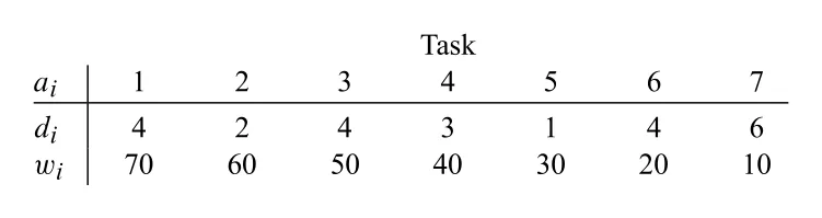 Figure 16.7 · PDF p. 467 · unit-time tasks의 deadlines와 penalties 예시
Figure 16.7의 tasks는 penalties 내림차순이 이미 a_1, a_2, ..., a_7 순서다. Greedy는 , , , 를 early set에 넣고, 와 은 넣으면 가 되어 deadline 4까지 5개 tasks를 끝내야 하므로 reject한다. 마지막 은 accept한다.
최종 optimal schedule은:
Early tasks는 <a_2, a_4, a_1, a_3, a_7>이고 late tasks는 , 이다. Total incurred penalty는:
Chapter 16 problem patterns
Chapter 16의 problems는 greedy가 맞는 경우와 DP가 필요한 경우를 구분하는 훈련이다.
| Problem | 핵심 패턴 |
|---|---|
| 16-1 Coin changing | U.S. coins나 powers of c에서는 greedy가 맞지만, 임의 coin denominations에서는 실패할 수 있어 DP가 필요하다. |
| 16-2 Scheduling to minimize average completion time | 모든 tasks가 동시에 available하면 shortest processing time first가 평균 completion time을 줄인다. Release time과 preemption이 있으면 shortest remaining processing time 계열이 필요하다. |
| 16-3 Acyclic subgraphs | Undirected graph의 acyclic edge sets는 graphic matroid와 연결된다. Directed acyclic edge sets는 일반적으로 matroid가 아닐 수 있다. |
| 16-4 Scheduling variations | Deadline 이전의 latest available slot에 high-penalty task를 배정하는 구현. Disjoint-set forest로 빈 slot을 빠르게 찾을 수 있다. |
| 16-5 Off-line caching | 미래 requests를 모두 알 때 furthest-in-future eviction이 optimal이다. Online caching과 달리 future information을 greedy choice에 쓴다. |
Chapter notes
Greedy algorithms와 matroids에 대한 더 많은 이론은 combinatorial optimization 문헌으로 이어진다. Matroid theory는 Whitney의 1935년 작업에서 시작되었고, greedy algorithm은 Edmonds의 1971년 combinatorial optimization 문헌에서 중요한 형태로 등장했다. Huffman codes는 1952년에 제안되었고, matroid theory를 더 일반화한 greedoid theory도 이후 발전했다.
연결 관계
| 연결 대상 | 관계 |
|---|---|
| Chapter 15 Dynamic Programming | Greedy와 DP 모두 optimal substructure를 쓰지만, DP는 subproblems를 먼저 풀고 greedy는 safe choice를 먼저 한다. |
| Chapter 6 Heapsort / priority queue | Huffman algorithm은 min-priority queue, EXTRACT-MIN, INSERT, BUILD-MIN-HEAP을 사용한다. |
| Chapter 21 Disjoint Sets | Scheduling variation에서 latest available slot을 빠르게 찾는 데 disjoint-set forest가 쓰인다. |
| Chapter 23 Minimum Spanning Trees | Graphic matroid와 weighted matroid greedy theorem은 MST greedy algorithms의 이론적 배경이 된다. |
| Chapter 24 Shortest Paths | Dijkstra’s algorithm은 greedy method의 대표 응용이다. |
| Chapter 35 Approximation Algorithms | Set cover greedy heuristic처럼 optimal 보장은 약하지만 greedy가 좋은 근사를 주는 사례로 이어진다. |
오해하기 쉬운 내용
| 오해 | 바로잡기 |
|---|---|
| Locally best면 항상 globally best다. | 아니다. Greedy-choice property를 별도로 증명해야 한다. 0-1 knapsack의 value density greedy가 반례다. |
| Optimal substructure가 있으면 greedy가 된다. | 아니다. DP와 greedy 모두 optimal substructure를 쓰지만, greedy는 safe first choice가 추가로 필요하다. |
| Activity-selection은 가장 짧은 activity를 고르면 된다. | 아니다. CLRS exercises가 duration, overlap count, earliest start time rules의 실패를 묻는다. |
| Huffman tree는 BST다. | 아니다. Characters는 leaves에 있고 sorted order는 중요하지 않다. |
| Matroid 이론이 모든 greedy algorithm을 설명한다. | 아니다. Activity-selection과 Huffman coding도 greedy지만 이 section의 matroid theory가 직접 포괄하지는 않는다. |
| Task scheduling에서 late tasks의 순서도 중요하다. | penalty는 late 여부만 보므로, early set이 정해지면 late tasks 순서는 penalty에 영향을 주지 않는다. |
면접 질문
greedy-choice property와optimal substructure의 차이를 activity-selection 예시로 설명하라.- Activity-selection에서 earliest finish time을 고르는 것이 safe한 이유를 exchange argument로 증명하라.
- 0-1 knapsack과 fractional knapsack 중 왜 하나만 value density greedy가 통하는가?
prefix code가 decoding을 unambiguous하게 만드는 이유는 무엇인가?- Huffman algorithm이 두 minimum-frequency nodes를 merge해도 되는 이유를 Lemma 16.2 관점에서 설명하라.
matroid의 hereditary property와 exchange property가 greedy correctness에 각각 어떻게 쓰이는가?- Graphic matroid에서 independent set은 무엇이고, maximal independent set은 무엇인가?
- Unit-time task scheduling with deadlines and penalties를 matroid problem으로 바꾸는 핵심 아이디어는 무엇인가?