Chapter 17. Amortized Analysis

개요

amortized analysis는 data structure operations의 sequence 전체를 보고, 한 operation당 평균적으로 얼마의 비용이 드는지 worst-case로 보장하는 분석 방법이다. 어떤 단일 operation은 비쌀 수 있지만, 그런 비싼 operation이 자주 일어나지 않는다면 전체 sequence의 평균 비용은 작을 수 있다.

중요한 점은 average-case analysis와 다르다는 것이다. Amortized analysis는 probability를 쓰지 않는다. 임의의 operation sequence에 대해 worst-case total cost를 upper bound하고, 그 total을 operations 수로 나누어 operation당 amortized cost를 얻는다.

Chapter 17의 세 가지 대표 기법은 다음과 같다.

방법	핵심 아이디어
`aggregate analysis`	`n` operations 전체 cost $T(n)$ 을 직접 bound하고, $T(n)/n$ 을 모든 operation의 amortized cost로 둔다.
`accounting method`	어떤 operations를 실제보다 비싸게 charge하고, 초과분을 prepaid credit으로 저장해 나중의 비싼 operations 비용을 지불한다.
`potential method`	credit을 개별 object가 아니라 data structure 전체의 potential energy $\Phi$ 로 저장한다.

분석 중 등장하는 charge, credit, potential은 코드에 넣는 값이 아니다. 분석을 위한 장부일 뿐이다.

핵심 개념

용어	뜻	검색 키워드
amortized cost	operation sequence 전체를 기준으로 operation당 나누어 본 보장 비용	amortized cost
aggregate analysis	전체 sequence의 total cost를 먼저 bound하는 amortized analysis 방법	aggregate analysis
accounting method	overcharge와 stored credit으로 비용을 설명하는 방법	accounting method
potential method	data structure state에 potential function을 정의해 비용을 설명하는 방법	potential method
actual cost	operation이 실제로 지불한 비용	actual cost
amortized analysis vs average-case	probability 없이 worst-case sequence 평균을 보장한다는 차이	average-case analysis
dynamic table	load factor에 따라 table을 expand/contract하는 table	dynamic table

세부 정리

17.1 Aggregate analysis

aggregate analysis에서는 모든 n에 대해 n operations sequence의 worst-case total cost가 $T(n)$ 임을 보인다. 그러면 operation당 amortized cost는 $T(n)/n$ 이다. 이 방식에서는 operation 종류가 여러 개여도 모두 같은 amortized cost를 부여한다.

Stack operations with MULTIPOP

기본 stack operations는 다음과 같다.

Operation	동작	Cost
`PUSH(S, x)`	object `x`를 stack top에 올림	1
$POP(S)$	stack top object를 제거하고 반환	1

여기에 MULTIPOP(S, k)를 추가한다. 이 operation은 stack top에서 최대 k개를 pop한다. Stack에 k개보다 적게 있으면 stack 전체를 비운다.

MULTIPOP(S, k)
1  while not STACK-EMPTY(S) and k > 0
2      POP(S)
3      k = k - 1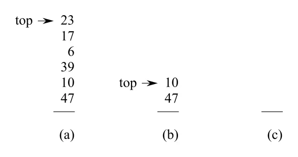

Figure 17.1 · PDF p. 474 · MULTIPOP이 stack top에서 여러 objects를 제거하는 과정

Stack size가 s일 때 MULTIPOP(S, k)의 actual cost는 loop iterations 수, 즉 min(s, k)다. 단일 MULTIPOP만 보면 worst-case cost가 $O(n)$ 일 수 있다. 그래서 각 operation의 individual worst-case만 단순히 더하면 n operations sequence가 $O(n^{2})$ 처럼 보인다.

하지만 이는 tight하지 않다. Initially empty stack에서 n개의 PUSH, POP, MULTIPOP operations를 수행한다고 하자. 어떤 object도 PUSH되기 전에는 pop될 수 없고, 한 번 pop된 object는 다시 stack에 들어가지 않는 한 다시 pop될 수 없다. 따라서 nonempty stack에서 실행되는 POP 호출 수는 전체 PUSH 수를 넘지 못하고, 전체 PUSH 수도 최대 n이다.

결론:

\begin{aligned} \text{total cost of n stack operations} &= O(n) \\ \text{amortized cost per operation} &= O(n) / n = O(1) \end{aligned}

즉 MULTIPOP 하나는 비쌀 수 있지만, sequence 전체에서 pop될 수 있는 objects 수가 push된 objects 수로 제한되므로 모든 stack operations의 amortized cost는 $O(1)$ 이다.

Binary counter

두 번째 예시는 k-bit binary counter다. Array $A[0..k-1]$ 에 bits를 저장하며, $A[0]$ 은 lowest-order bit, $A[k-1]$ 은 highest-order bit다.

Counter value는:

x = \sum_{i=0}^{k-1} A[i] \cdot 2^{i}

초기값은 0이고 모든 bits가 0이다. $INCREMENT(A)$ 는 counter에 1을 더한다.

INCREMENT(A)
1  i = 0
2  while i < A.length and A[i] == 1
3      A[i] = 0
4      i = i + 1
5  if i < A.length
6      A[i] = 1

While loop는 trailing 1s를 0으로 바꾸며 carry를 전달한다. 처음 만나는 0 bit를 1로 바꾸면 increment가 끝난다. Operation cost는 flipped bits 수에 비례한다.

단일 INCREMENT의 worst-case는 counter가 all 1s일 때 $\Theta(k)$ 다. 따라서 단순 worst-case 곱셈으로는 n increments가 $O(nk)$ 처럼 보인다. 하지만 aggregate analysis로는 훨씬 작다.

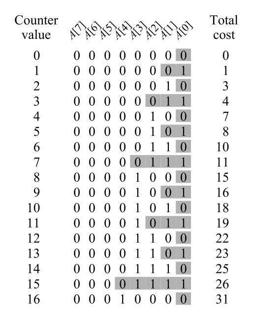Figure 17.2 · PDF p. 476 · 8-bit binary counter에서 16번 INCREMENT 동안 flip되는 bits와 누적 cost

Bit별 flip 빈도를 보면:

Bit	Flip frequency in `n` increments
$A[0]$	`n`번
$A[1]$	$\lfloor n/2 \rfloor$ 번
$A[2]$	$\lfloor n/4 \rfloor$ 번
$A[i]$	$\lfloor n/2^{i} \rfloor$ 번

따라서 전체 flips 수는:

\begin{aligned} \sum_{i=0}^{k-1} \lfloor n / 2^{i} \rfloor \\ < n \sum_{i=0}^{\infty} 1/2^{i} \\ = 2n \end{aligned}

즉 initially zero counter에서 n번 INCREMENT를 수행하는 worst-case total cost는 $O(n)$ 이고, amortized cost per INCREMENT는 $O(1)$ 이다.

Aggregate analysis의 핵심 감각

Aggregate analysis는 “비싼 operation이 있다”는 사실을 부정하지 않는다. 대신 sequence 전체에서 그 비싼 일이 얼마나 자주 누적될 수 있는지 직접 센다.

예	비싼 단일 operation	전체 sequence에서 제한되는 이유
`MULTIPOP`	stack에 많이 쌓인 objects를 한 번에 pop하면 비쌈	pop될 object는 이전에 push되어 있어야 하며, 각 push당 pop은 최대 한 번
binary counter	many trailing 1s가 한 번에 flip되면 비쌈	높은 bit일수록 flip 빈도가 기하급수적으로 줄어듦

이 구간의 결론은 “individual worst-case를 단순히 operations 수만큼 곱하면 overly pessimistic할 수 있다”는 것이다. Amortized analysis는 data structure의 state 변화가 비싼 operations의 빈도를 제한한다는 사실을 이용한다.

17.2 The accounting method

accounting method는 operation마다 amortized cost를 직접 charge하고, 실제 비용보다 더 많이 받은 금액을 data structure 안의 특정 objects에 credit으로 저장하는 방식이다. 나중에 실제 비용이 charge보다 큰 operation이 오면 저장된 credit으로 부족분을 지불한다.

Aggregate analysis와 달리 accounting method에서는 operation 종류마다 서로 다른 amortized cost를 줄 수 있다. 핵심 제약은 total amortized cost가 항상 total actual cost의 upper bound여야 한다는 것이다.

Accounting invariant

$c_{i}$ 를 i번째 operation의 actual cost, ĉ_i를 amortized cost라고 하자. 모든 operation sequence와 모든 prefix length n에 대해 다음이 성립해야 한다.

\sum_{i=1}^{n} ĉ_{i} \ge \sum_{i=1}^{n} c_{i} (17.1)

두 합의 차이가 data structure에 저장된 total credit이다.

\text{total credit} = \sum amortized costs - \sum actual costs

따라서 분석 중 어떤 시점에도 total credit이 negative가 되면 안 된다. 초반 operations를 과소 charge하고 나중에 갚겠다고 하면, 그 prefix sequence에서는 amortized total이 actual total보다 작아져 upper bound가 깨진다.

Stack operations accounting

Stack example에서 actual costs는 다음과 같다.

Operation	Actual cost
`PUSH`	1
`POP`	1
`MULTIPOP`	`min(k, s)`

Accounting method에서는 다음 amortized costs를 부여한다.

Operation	Amortized cost
`PUSH`	2
`POP`	0
`MULTIPOP`	0

PUSH를 할 때 2 dollars를 charge한다고 생각하자. 1 dollar는 actual push cost를 지불하고, 남은 1 dollar는 새로 push된 object 위에 credit으로 둔다. 그러면 stack 위의 모든 object는 항상 1 dollar credit을 가지고 있다.

POP은 amortized cost가 0이지만, pop되는 object 위의 1 dollar credit으로 actual pop cost를 지불한다. MULTIPOP도 마찬가지다. 여러 objects를 pop할 때 각 object가 자기 위의 credit으로 자신의 pop cost를 지불한다.

불변식은 다음과 같다.

\begin{aligned} \text{credit on each object currently in stack} &= 1 \\ \text{total credit} &= current stack size \ge 0 \end{aligned}

따라서 어떤 sequence에서도 total credit은 negative가 되지 않는다. n operations의 total amortized cost는 PUSH마다 2, 나머지는 0이므로 $O(n)$ 이고, 이 값이 total actual cost를 upper bound한다.

Binary counter accounting

Binary counter에서는 bit flip 하나를 cost 1로 본다. Accounting method는 bit를 $0 \to 1$ 로 set할 때 2 dollars를 charge한다.

Bit transition	Charge	실제 지불	저장/사용
$0 \to 1$	2	1	남은 1 dollar를 그 bit 위에 credit으로 저장
$1 \to 0$	0	1	bit 위의 1 dollar credit으로 reset 비용 지불

이때 invariant는 다음과 같다.

\begin{aligned} \text{every bit whose value is 1 has 1 dollar of credit} \\ \text{total credit} &= number of 1s in the counter \ge 0 \end{aligned}

INCREMENT 중 while loop에서 trailing 1s를 0으로 바꾸는 비용은 각 1 bit 위의 credit으로 지불한다. 마지막에 line 6에서 새 0 bit를 1로 set하는 경우가 있어도, 한 번의 INCREMENT가 새로 set하는 bit는 많아야 하나다. 따라서 INCREMENT의 amortized cost는 최대 2다.

결론:

\begin{aligned} \text{amortized cost per INCREMENT} &\le 2 = O(1) \\ \text{total actual cost of } n \text{ INCREMENT operations} &\le \text{total amortized cost} = O(n) \end{aligned}

Accounting method의 설계 요령

Accounting method는 “비싼 future operation을 어떤 earlier cheap operation이 미리 지불할 수 있는가?”를 찾는 방식이다.

예	Overcharged operation	저장 위치	나중에 지불하는 비용
stack	`PUSH`	pushed object	future `POP` 또는 `MULTIPOP`에서 object를 제거하는 비용
binary counter	bit $0 \to 1$ set	bit value가 1인 position	future $1 \to 0$ reset 비용

좋은 accounting scheme은 credit의 위치와 사용처가 명확해야 한다. “총합으로는 될 것 같다”가 아니라, 어떤 object에 얼마가 저장되어 있고 어떤 operation이 그 credit을 쓰는지 설명할 수 있어야 한다.

17.3 The potential method

potential method는 prepaid work를 특정 object의 credit으로 두지 않고, data structure 전체의 potential energy, 즉 potential로 저장한다. 어떤 operation이 potential을 증가시키면 미래 비용을 미리 저축한 것이고, potential을 감소시키면 저장된 potential로 실제 비용 일부를 지불한 것이다.

Potential function and amortized cost

초기 data structure를 $D_{0}$ 라고 하자. i번째 operation 후의 data structure를 $D_{i}$ , actual cost를 $c_{i}$ 라고 한다. Potential function $\Phi$ 는 각 data structure state $D_{i}$ 를 real number $\Phi(D_{i})$ 로 보낸다.

Potential method에서 i번째 operation의 amortized cost ĉ_i는 다음과 같다.

ĉ_{i} = c_{i} + \Phi(D_{i}) - \Phi(D_{i-1}) (17.2)

즉:

\text{amortized cost} = actual cost + change in potential

n operations 전체에 대해 합을 취하면 potential terms가 telescoping된다.

\begin{aligned} \sum_{i=1}^{n} ĉ_{i} \\ = \sum_{i=1}^{n} (c_{i} + \Phi(D_{i}) - \Phi(D_{i-1})) \\ = \sum_{i=1}^{n} c_{i} + \Phi(D_{n}) - \Phi(D_{0}) (17.3) \end{aligned}

따라서 $\Phi(D_{n}) \ge \Phi(D_{0})$ 이면:

\sum amortized costs \ge \sum actual costs

실제로는 operations 수를 미리 모르는 경우가 많으므로, 보통 $\Phi(D_{0}) = 0$ 으로 정의하고 모든 i에 대해 $\Phi(D_{i}) \ge 0$ 임을 보인다. 그러면 모든 prefix sequence에 대해 amortized total이 actual total의 upper bound가 된다.

Potential difference의 의미는 다음과 같다.

$\Phi(D_{i}) - \Phi(D_{i-1})$	의미
positive	operation을 overcharge하고 potential을 쌓음
zero	amortized cost와 actual cost가 같음
negative	potential을 꺼내 actual cost를 보조함

Potential function은 하나만 정답인 것이 아니다. 어떤 $\Phi$ 를 잡느냐에 따라 amortized bounds가 달라질 수 있고, 좋은 potential function은 자료구조가 “비싼 operation 직전까지 얼마나 에너지를 모았는가”를 잘 표현한다.

Stack operations with potential

Stack의 potential을 현재 stack 안의 objects 수로 정의한다.

\Phi(D_{i}) = number of objects in stack after i-th operation

Initially empty stack이므로 $\Phi(D_{0}) = 0$ 이고, stack size는 음수가 될 수 없으므로 모든 i에 대해 $\Phi(D_{i}) \ge 0$ 이다.

PUSH 직전 stack size가 s라면:

\begin{aligned} \text{actual cost} &= 1 \\ \Phi(D_{i}) - \Phi(D_{i-1}) &= (s+1) - s = 1 \\ ĉ_{i} &= 1 + 1 = 2 \end{aligned}

MULTIPOP(S, k)가 실제로 $k' = \min(k, s)$ 개를 pop한다고 하자.

\begin{aligned} \text{actual cost} &= k' \\ \Phi(D_{i}) - \Phi(D_{i-1}) &= -k' \\ ĉ_{i} &= k' - k' = 0 \end{aligned}

Ordinary POP도 $k'=1$ 인 경우와 같으므로 amortized cost가 0이다. 따라서 stack operations의 amortized costs는:

Operation	Amortized cost by potential
`PUSH`	2
`POP`	0
`MULTIPOP`	0

Accounting method에서 “object마다 1 credit”을 두었던 것과 같은 분석을, potential method에서는 “stack size 전체가 potential”이라고 표현한 셈이다.

Binary counter with potential

Binary counter에서는 potential을 counter 안의 1 bits 수로 둔다.

\Phi(D_{i}) = b_{i} = number of 1s after i-th INCREMENT

i번째 INCREMENT가 $t_{i}$ 개의 1 bits를 0으로 reset한다고 하자. 그 뒤 최대 하나의 bit를 1로 set하므로 actual cost는:

c_{i} \le t_{i} + 1

Reset된 $t_{i}$ 개의 1 bits 때문에 potential은 줄고, 새로 set되는 bit 때문에 많아야 1 증가한다.

\begin{aligned} b_{i} &\le b_{i-1} - t_{i} + 1 \\ \Phi(D_{i}) - \Phi(D_{i-1}) &\le 1 - t_{i} \end{aligned}

따라서 amortized cost는:

\begin{aligned} ĉ_{i} &= c_{i} + \Phi(D_{i}) - \Phi(D_{i-1}) \\ &\le (t_{i} + 1) + (1 - t_{i}) \\ &= 2 \end{aligned}

Counter가 0에서 시작하면 $\Phi(D_{0}) = 0$ , 그리고 항상 $\Phi(D_{i}) \ge 0$ 이므로 n번 INCREMENT의 total actual cost는 $O(n)$ 이다.

Counter가 0에서 시작하지 않는 경우

Potential method는 초기 state가 0이 아닐 때도 깔끔하다. Counter가 처음에 $b_{0}$ 개의 1 bits를 가지고, n operations 후 $b_{n}$ 개의 1 bits를 가진다고 하자. Equation (17.3)을 actual cost 기준으로 재배열하면:

\sum_{i=1}^{n} c_{i} = \sum_{i=1}^{n} ĉ_{i} - \Phi(D_{n}) + \Phi(D_{0}) (17.4)

각 $ĉ_{i} \le 2$ , $\Phi(D_{0})=b_{0}$ , $\Phi(D_{n})=b_{n}$ 이므로:

\sum c_{i} \le 2n - b_{n} + b_{0}

특히 $b_{0} \le k$ 이고 $k = O(n)$ 이면 total actual cost는 여전히 $O(n)$ 이다. 더 일반적으로 충분히 많은 increments를 수행해 초기 1 bits가 만들어 둔 potential 효과가 희석되면 amortized bound가 유지된다.

Accounting method와 potential method의 차이

관점	Accounting method	Potential method
credit 저장 위치	특정 object에 저장	data structure state 전체에 저장
핵심 조건	total credit never negative	$\Phi(D_{i}) \ge \Phi(D_{0})$ 또는 $\Phi(D_{i}) \ge 0$
계산 방식	operation별 charge와 credit 사용 설명	$c_{i} + \Delta\Phi$ 로 수식 계산
장점	직관적이고 object-level explanation이 좋음	복잡한 structure나 resizing처럼 전체 상태를 다룰 때 강력함

Potential method는 17.4의 dynamic tables 분석에서 특히 유용하다. Table이 거의 가득 찰수록 expansion 비용을 낼 potential이 쌓이고, deletion까지 고려할 때는 load factor가 너무 낮아지는 상황까지 함께 표현해야 한다.

17.4 Dynamic tables

Dynamic tables는 저장해야 할 object 수를 미리 알 수 없을 때 table 크기를 자동으로 조절하는 문제다. 너무 작으면 새 object를 넣을 공간이 없고, 너무 크면 unused space가 낭비된다. 목표는 TABLE-INSERT와 TABLE-DELETE를 지원하면서도 각 operation의 amortized cost를 $O(1)$ 로 유지하는 것이다.

이 절에서 table T는 다음 값을 가진다.

표기	의미
`T.table`	실제 slot array
`T.num`	현재 저장된 object 수
`T.size`	현재 table의 slot 수
$\alpha(T) = T.num / T.size$	`load factor`

비어 있지 않은 table에서는 $\alpha(T)=T.num/T.size$ 이고, empty table에서는 편의상 $T.size=0$ , $\alpha(T)=1$ 로 둔다. load factor가 어떤 positive constant 아래로 떨어지지 않도록 보장하면 unused space는 전체 table size의 constant fraction 안에 묶인다.

17.4.1 Table expansion

먼저 deletion이 없고 insertion만 있다고 하자. Table이 가득 찬 상태( $T.num = T.size$ , 즉 $\alpha(T)=1$ )에서 새 object를 넣으려면 더 큰 table을 새로 allocate하고 기존 object를 모두 copy한 뒤 old table을 free해야 한다. 가장 흔한 전략은 table size를 두 배로 늘리는 doubling이다.

TABLE-INSERT(T, x)
1  if T.size == 0
2      allocate T.table with 1 slot
3      T.size = 1
4  if T.num == T.size
5      allocate new-table with 2 * T.size slots
6      insert all items in T.table into new-table
7      free T.table
8      T.table = new-table
9      T.size = 2 * T.size
10 insert x into T.table
11 T.num = T.num + 1

expansion은 line 5-9의 재할당과 copy 과정이다. Cost model은 한 object 삽입 비용을 1로 보고, allocation/free overhead는 copied objects 수에 의해 dominate된다고 본다. 따라서 i번째 insertion이 expansion을 일으키지 않으면 $c_{i}=1$ 이고, expansion을 일으키면 기존 $i-1$ 개를 copy하고 새 item을 insert하므로 $c_{i}=i$ 가 된다.

Doubling 전략의 핵심은 expansion이 드물다는 점이다. i번째 insert 직전에 table이 full이려면 $i-1$ 이 정확히 2의 거듭제곱이어야 한다. 그러므로 n번 insert의 total actual cost는:

\begin{aligned} \sum_{i=1}^{n} c_{i} \\ &\le n + \sum_{j=0}^{\lfloor \lg n \rfloor} 2^{j} \\ &< 3n \end{aligned}

따라서 TABLE-INSERT의 amortized cost는 at most 3, 즉 $O(1)$ 이다. Worst-case single insertion은 expansion 때문에 $\Theta(n)$ 일 수 있지만, 긴 sequence 전체에서는 expensive operation이 충분히 sparse하게 나타난다.

Accounting method로도 같은 결론을 볼 수 있다. 각 insertion에 $3을 charge한다. $1은 지금 item을 실제로 insert하는 데 쓰고, $1은 새 item이 다음 expansion 때 copy될 비용으로 저장하고, 나머지 $1은 이미 한 번 copy되어 들어온 old item들 중 하나의 다음 copy 비용으로 저장한다. Expansion 직후 table은 half full이므로 다음 expansion까지 들어오는 insertions가 충분한 credit을 쌓아 준다.

Potential method에서는 다음 potential function을 둔다.

\Phi(T) = 2 \cdot T.num - T.size (17.5)

Insertion만 있는 경우 table은 항상 at least half full이므로 $\Phi(T) \ge 0$ 이다. Expansion 직후에는 $T.num = T.size/2$ 라서 $\Phi(T)=0$ 이고, table이 full에 가까워질수록 potential이 커진다. 이 potential은 “다음 expansion에서 copy 비용으로 쓸 에너지”를 table state에 저장해 두는 역할을 한다.

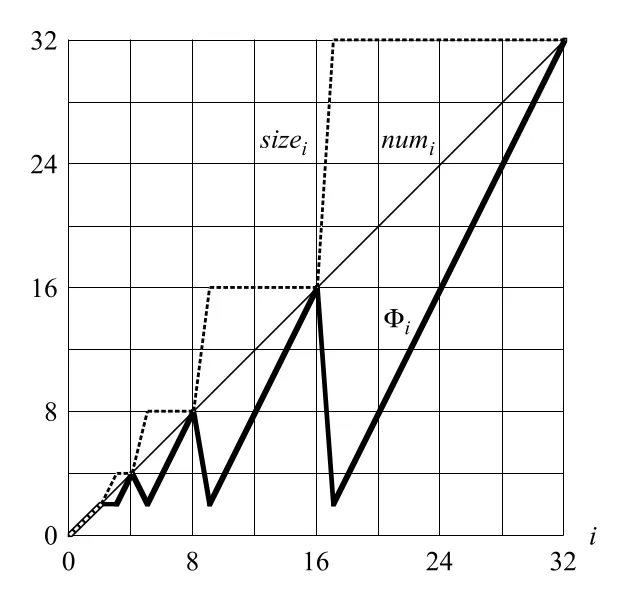Figure 17.3 · PDF p. 488 · insert-only dynamic table에서 num, size, potential 변화

Amortized cost 계산은 두 경우로 나뉜다.

경우	Actual cost $c_{i}$	Potential change	Amortized cost
expansion 없음	`1`	`+2`	`3`
expansion 있음	$T.num_{i-1}+1$	`2 - T.num_i`에 해당하도록 감소	`3`

즉 expansion이 일어나는 순간 actual cost는 크지만, 직전에 쌓여 있던 potential이 크게 감소해서 amortized cost는 constant로 유지된다.

17.4.2 Table expansion and contraction

Deletion까지 지원하려면 table이 지나치게 비었을 때 contraction도 해야 한다. 하지만 단순히 “full이면 double, delete 후 half보다 작아지면 halve”로 하면 좋지 않다. Table size가 $n/2$ 이고 full인 상태에서 insert 한 번으로 size n으로 expand된 뒤, delete 몇 번으로 곧바로 size $n/2$ 로 contract될 수 있다. 그 다음 insert들이 다시 expansion을 일으키면 expansion/contraction이 반복되어 $\Theta(n)$ cost operation이 연속적으로 발생하고, n operations가 $\Theta(n^{2})$ total cost까지 커질 수 있다.

해결책은 expansion과 contraction 사이에 간격을 두는 hysteresis다.

상황	동작
$\alpha(T)=1$ 에서 insert	table size를 double
delete 후 $\alpha(T) < 1/4$	table size를 halve
그 외	size 유지

이 정책에서는 expansion이나 contraction 직후 load factor가 대략 $1/2$ 로 돌아온다. 또한 nonempty table의 load factor는 항상 at least $1/4$ 이므로 unused space도 constant factor 안에 묶인다.

Insertion-only potential $2T.num - T.size$ 는 $\alpha < 1/2$ 에서 negative가 될 수 있으므로 deletion을 함께 분석하려면 potential을 바꿔야 한다. 책은 다음 piecewise potential을 사용한다.

\Phi(T) = \begin{cases} 2 \cdot T.\mathrm{num} - T.\mathrm{size}, & \text{if } \alpha(T) \ge 1/2\\ T.\mathrm{size}/2 - T.\mathrm{num}, & \text{if } \alpha(T) < 1/2 \end{cases} \qquad (17.6)

이 potential은 $\alpha=1/2$ 에서 0이고, table이 full에 가까워질수록 expansion 비용을 위해 증가하며, table이 $1/4$ 에 가까워질수록 contraction 비용을 위해 증가한다. Empty table에서도 $\Phi(T)=0$ 으로 두며, 모든 state에서 nonnegative다.

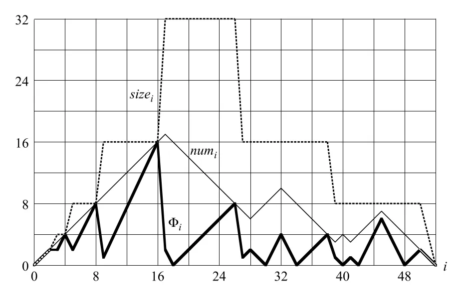Figure 17.4 · PDF p. 490 · expansion/contraction dynamic table의 piecewise potential

Amortized analysis는 operation 직전과 직후의 load factor에 따라 나뉜다.

Operation	조건	핵심 결론
`TABLE-INSERT`	$\alpha_{i-1} \ge 1/2$	17.4.1과 같은 방식으로 amortized cost $\le 3$
`TABLE-INSERT`	$\alpha_{i-1} < 1/2$ , 여전히 $\alpha_{i} < 1/2$	actual cost 1이지만 potential이 1 감소해 amortized cost 0
`TABLE-INSERT`	$\alpha_{i-1} < 1/2$ , insertion 후 $\alpha_{i} \ge 1/2$	경계 $1/2$ 을 넘는 순간에도 amortized cost는 constant, 실제 계산상 $< 3$
`TABLE-DELETE`	$\alpha_{i-1} < 1/2$ , contraction 없음	actual cost 1과 potential 증가를 합쳐 amortized cost 2
`TABLE-DELETE`	deletion 후 contraction 발생	delete 1개 + `T.num_i`개 copy가 actual cost지만, potential 감소가 이를 상쇄해 amortized cost 1

Contraction이 발생하는 delete에서는 deletion 직후 object 수를 T.num_i라고 하면 새 table size와 기존 table size 사이에 다음 관계가 성립한다.

T.size_{i} / 2 = T.size_{i-1} / 4 = T.num_{i} + 1

즉 contraction 직전에는 table이 $1/4$ threshold를 막 지나고 있었고, contraction 후에는 load factor가 다시 약 $1/2$ 가 된다. 이 순간 potential이 크게 줄어 expensive copying을 지불한다. $\alpha_{i-1} \ge 1/2$ 인 delete의 상세 계산은 연습문제로 남겨져 있지만, 같은 potential로 constant amortized bound가 나온다.

결론적으로 doubling과 quarter-threshold contraction을 쓰는 dynamic table은 임의의 n개 TABLE-INSERT, TABLE-DELETE sequence에 대해 total actual cost $O(n)$ , per-operation amortized cost $O(1)$ 을 보장한다.

Dynamic table 분석의 설계 포인트

설계 선택	이유
Full에서 `double`	expansion 이후 load factor를 $1/2$ 로 만들어 다음 expansion까지 충분한 insertions를 확보
$1/2$ 아래에서 바로 halve하지 않음	insert/delete가 threshold 주변에서 반복될 때 thrashing 방지
$1/4$ 아래에서 `halve`	unused space를 constant factor로 제한하면서 contraction 사이에 충분한 deletions 확보
Piecewise potential	full 쪽 expansion 비용과 sparse 쪽 contraction 비용을 하나의 함수로 동시에 표현

여기서 중요한 trade-off는 space와 resizing frequency다. Threshold를 너무 높게 잡으면 table이 자주 줄어 thrashing 위험이 커지고, 너무 낮게 잡으면 unused space가 커진다. CLRS의 $1/4$ contraction threshold는 proof가 단순하면서도 constant amortized bound와 constant space overhead를 함께 만족하는 대표적인 선택이다.

Problems와 chapter notes의 연결

이 장의 마지막 problems는 amortized analysis가 단순 resizing을 넘어 다양한 자료구조와 알고리즘에서 어떻게 쓰이는지 보여 준다.

항목	연결되는 아이디어
`17-1 Bit-reversed binary counter`	`FFT`의 `bit-reversal permutation`처럼 unusual increment pattern도 bit flip 총량을 amortized하게 분석할 수 있음
`17-2 Making binary search dynamic`	크기가 2의 거듭제곱인 여러 sorted arrays를 binary carry처럼 merge해 search $O(\lg^{2} n)$ , insertion amortized $O(\lg n)$ 을 얻는 구조
`17-3 Amortized weight-balanced trees`	subtree가 $\alpha-balanced$ 조건을 깨면 rebuild하고, imbalance가 쌓이는 정도를 potential로 해석
`17-4 The cost of restructuring red-black trees`	한 operation에 color changes는 많을 수 있지만 rotations 같은 structural modifications는 sequence 전체에서 amortized $O(1)$ 로 제어 가능
`17-5 Competitive analysis of self-organizing lists`	`move-to-front` heuristic을 offline optimum과 비교하며, inversions를 potential처럼 사용

Chapter notes는 amortized라는 용어와 이 분석 방식이 Sleator와 Tarjan의 연구에서 체계화되었음을 언급한다. Potential method는 upper bound뿐 아니라 lower bound에도 쓰일 수 있고, 이후 Chapter 21의 disjoint-set forest 분석에서도 더 정교한 potential argument가 등장한다.

연결 관계

연결 대상	관계
Chapter 6 `heapsort`	배열 기반 tree 표현처럼 구조 유지 비용을 operation sequence로 보는 관점이 이어짐
Chapter 10 `stacks`	`MULTIPOP` 예시는 stack ADT의 operation sequence 비용을 다시 해석함
Chapter 13 `red-black trees`	balancing operation의 worst-case와 sequence-level cost를 구분하는 관점이 중요함
Chapter 14 `augmenting data structures`	추가 metadata를 유지하는 비용이 operation sequence에서 어떻게 분산되는지 분석할 때 amortized reasoning이 유용함
Chapter 21 `disjoint-set forests`	CLRS에서 가장 정교한 amortized analysis 중 하나로 이어짐

오해하기 쉬운 내용

오해	정정
Amortized analysis는 average-case analysis다	아니다. Probability나 input distribution 없이 worst-case operation sequence 전체의 평균 비용을 bound한다
어떤 operation도 실제로 싸다는 뜻이다	아니다. 개별 operation은 $\Theta(n)$ 일 수 있지만, 그런 operation이 자주 반복될 수 없음을 보인다
Accounting method의 credit은 실제 메모리나 필드다	분석을 위한 가상 장부일 뿐이며 implementation에 저장할 필요가 없다
Potential function은 아무 nonnegative 함수면 된다	$c_{i} + \Delta\Phi$ 가 원하는 bound를 주도록 state 변화와 잘 맞아야 한다
Dynamic table은 half 미만이면 바로 줄이면 된다	threshold 주변에서 expansion/contraction thrashing이 생길 수 있으므로 hysteresis가 필요하다

면접 질문

amortized analysis와 average-case analysis의 차이를 설명하라.
Stack의 MULTIPOP이 single operation으로는 $O(n)$ 인데 sequence에서는 amortized $O(1)$ 인 이유는 무엇인가?
Binary counter INCREMENT에서 total bit flips가 $O(n)$ 인 이유를 aggregate analysis로 설명하라.
Accounting method에서 amortized cost가 actual cost보다 작을 수 있는 이유와 필요한 invariant는 무엇인가?
Potential method의 식 $ĉ_{i} = c_{i} + \Phi(D_{i}) - \Phi(D_{i-1})$ 가 왜 telescoping되는가?
Dynamic table에서 doubling만 사용할 때 insertion의 amortized cost가 $O(1)$ 인 이유를 설명하라.
Dynamic table deletion에서 $1/2$ threshold로 바로 halve하면 왜 thrashing이 생기는가?
Expansion/contraction을 함께 지원하는 dynamic table의 potential function (17.6)이 왜 piecewise인지 설명하라.