개요
Indexing은 relation file 전체를 scan하지 않고 원하는 record 또는 record set을 빠르게 찾기 위해 file에 붙이는 보조 구조다. Chapter 13이 record와 file을 block/page에 어떻게 배치할지 다루었다면, Chapter 14는 그 file 위에 ordered index, B+ tree index, hash index, bitmap index, write-optimized index structure, spatial/temporal index를 얹어 access path를 만드는 방법을 다룬다.
이 장의 핵심은 “모든 index는 read 성능을 사는 대신 write/update와 space overhead를 지불한다”는 점이다. 어떤 index가 좋은지는 equality search, range search, insertion/deletion frequency, storage overhead, sequential scan 가능성, query workload에 따라 달라진다.
핵심 개념
index는 search-key value를 record location 또는 record pointer set에 연결하는 access path다.search key는 index lookup에 쓰는 attribute 또는 attribute set이며, primary key/candidate key/superkey와 다른 의미다.ordered index는 search-key values를 sorted order로 유지해 equality search와 range search를 지원한다.hash index는 hash function으로 bucket을 선택해 equality search를 빠르게 하지만 range search에는 약하다.clustering index또는primary index는 file의 physical/sequential order와 같은 search key order를 사용한다.nonclustering index또는secondary index는 file의 physical order와 다른 search key order를 사용한다.dense index는 모든 search-key value에 entry를 두고,sparse index는 일부 search-key value에만 entry를 둔다.multilevel index는 큰 index 위에 sparse outer index를 반복적으로 얹어 random I/O 수를 줄인다.composite search key는 둘 이상의 attributes로 구성된 search key이며 lexicographic ordering으로 정렬된다.
세부 정리
14.1 Basic Concepts
Database index는 책의 색인과 같은 역할을 한다. 특정 word/topic을 책 뒤 index에서 찾고 해당 page로 이동하듯, DBMS는 student.ID = 22201 같은 조건을 index에서 찾아 해당 record가 있는 disk block을 가져온다.
Index가 없으면 “Physics department의 모든 instructors 찾기”처럼 일부 records만 필요한 query도 relation 전체를 읽어야 한다. 이런 full scan은 single record lookup이나 특정 student의 takes records처럼 작은 subset을 찾는 query에서 특히 비싸다.
단순히 sorted list로 index를 만들면 큰 database에서 세 문제가 생긴다.
| 문제 | 이유 |
|---|---|
| index size | index 자체가 매우 커질 수 있다. |
| search time | sorted list라도 큰 index에서 disk block 탐색 비용이 남는다. |
| update cost | insert/delete 때 sorted order 유지 비용이 크다. |
그래서 DBMS는 workload에 따라 여러 indexing technique을 사용한다. 큰 분류는 다음 두 가지다.
| 종류 | 핵심 아이디어 | 강한 access type |
|---|---|---|
ordered indices | search-key values를 sorted order로 유지한다. | equality search, range search |
hash indices | hash function으로 search-key value를 bucket에 분배한다. | equality search |
Indexing technique을 평가할 때는 다음 기준을 본다.
| 평가 기준 | 질문 |
|---|---|
access types | 특정 값 lookup, range lookup 등 어떤 access를 빠르게 지원하는가 |
access time | 원하는 item 또는 item set을 찾는 데 얼마나 걸리는가 |
insertion time | 새 data item 위치를 찾고 index를 갱신하는 비용은 얼마인가 |
deletion time | 삭제 대상 찾기와 index 구조 갱신 비용은 얼마인가 |
space overhead | index가 차지하는 추가 공간은 적절한가 |
한 file에는 여러 index가 있을 수 있다. 예를 들어 책을 author, subject, title로 찾듯 relation도 여러 attributes로 찾을 수 있다. 이때 index lookup에 쓰는 attribute 또는 attribute set을 search key라고 한다. 여기서 key는 primary key, candidate key, superkey의 key와 다르다. Search key는 중복될 수 있고, 유일성을 보장하지 않아도 된다.
14.2 Ordered Indices
ordered index는 특정 search key에 대해 search-key values를 sorted order로 저장하고, 각 value를 그 value를 가진 record와 연결한다. File 자체도 어떤 search key 순서로 저장될 수 있고, file에는 서로 다른 search key에 대한 여러 index가 있을 수 있다.
clustering index와 secondary index
File이 sequentially ordered되어 있을 때, 그 file의 sequential order를 정의하는 search key에 대한 index를 clustering index라고 한다. Clustering index는 primary index라고도 불리지만, 반드시 primary key 위에 만들어진다는 뜻은 아니다. Search key가 file의 physical/sequential order를 정의하면 clustering index다.
반대로 file의 physical order와 다른 search key order를 사용하는 index는 nonclustering index 또는 secondary index다. clustered/nonclustered라는 표현도 같은 맥락에서 쓰인다.
index-sequential file은 search key로 sequentially ordered된 file과 그 search key 위의 clustering index를 함께 사용하는 구조다. 전체 file의 sequential processing과 individual record의 random access가 모두 필요한 application을 위해 설계된 오래된 indexing scheme이다.
14.2.1 Dense and Sparse Indices
index entry 또는 index record는 search-key value와 pointer로 구성된다. Record pointer는 보통 disk block identifier와 block 내부 offset으로 record를 식별한다.
dense index는 file에 나타나는 모든 search-key value마다 index entry를 둔다.
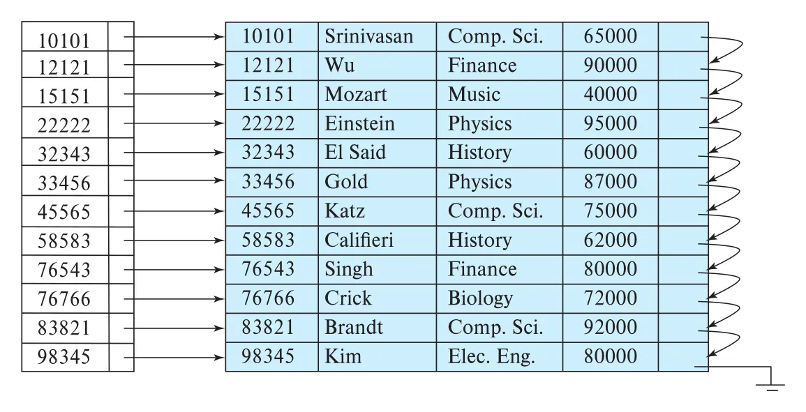 Figure 14.2 · PDF p. 656 · 모든 ID search-key value에 entry를 둔 dense index
Dense clustering index에서는 index entry가 search-key value와 그 value를 가진 첫 data record pointer를 가진다. 같은 search-key value의 나머지 records는 file이 같은 key order로 정렬되어 있으므로 sequentially 뒤에 놓인다. Dense nonclustering index에서는 같은 search-key value를 가진 모든 records가 file 여기저기에 있을 수 있으므로 pointer list가 필요하다.
sparse index는 일부 search-key values에만 index entry를 둔다. Sparse index는 relation이 search key 순서로 저장되어 있을 때, 즉 clustering index일 때만 사용할 수 있다.
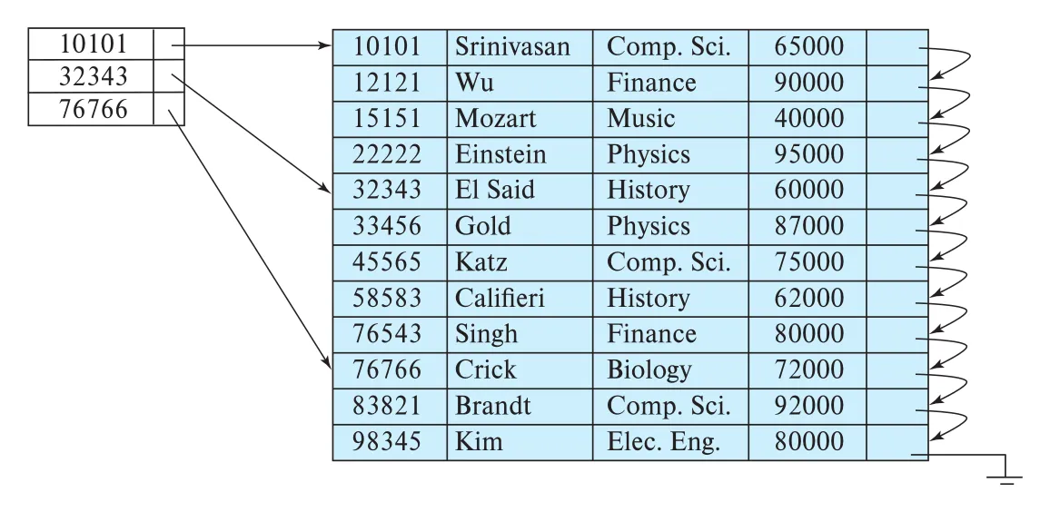 Figure 14.3 · PDF p. 656 · 일부 search-key value만 entry로 보관하고 data file을 이어서 scan하는 sparse index
Sparse index lookup은 찾는 value 이하의 가장 큰 search-key value entry를 찾고, 그 entry가 가리키는 record부터 sequential scan을 진행한다. 예를 들어 22222를 찾는데 sparse index에 22222가 없고 그보다 작은 마지막 entry가 10101이면, 10101이 가리키는 위치부터 file을 순차적으로 읽어 22222를 찾는다.
Dense index는 보통 record를 더 빨리 찾지만 space와 maintenance overhead가 크다. Sparse index는 느릴 수 있지만 작고 insert/delete 부담이 작다. 좋은 절충은 block마다 하나의 sparse index entry를 두는 것이다. Database request의 지배적 비용은 disk block을 memory로 가져오는 시간이므로, block 안 scan 비용은 상대적으로 작다. Block마다 entry를 두면 원하는 record가 들어 있는 block을 찾는 데 필요한 I/O를 줄이면서 index 크기도 줄인다.
14.2.2 Multilevel Indices
Index도 커지면 disk에 저장되는 sequential file이 된다. 예를 들어 1,000,000 tuples에 dense index를 만들고 4 KB block 하나에 100 index entries가 들어간다면, index는 10,000 blocks가 된다. 이 index 전체가 memory에 없다면 index lookup 자체가 여러 disk I/O를 일으킨다.
Index file에 binary search를 적용할 수는 있지만, b index blocks에 대해 최대 ceil(log2(b)) random block reads가 필요하다. 10,000 blocks면 14 random reads다. Magnetic disk에서 random read가 10 ms라면 single index search가 140 ms가 되어 초당 검색 수가 크게 제한된다.
해결책은 index를 또 하나의 ordered file로 보고, original index인 inner index 위에 sparse outer index를 만드는 것이다.
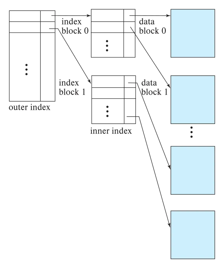 Figure 14.5 · PDF p. 658 · inner index 위에 sparse outer index를 얹은 two-level sparse index
Lookup은 outer index에서 원하는 search-key value 이하의 가장 큰 entry를 찾고, 그 pointer가 가리키는 inner index block을 읽은 뒤, 그 block 안에서 다시 적절한 entry를 찾아 data file block으로 이동한다. Outer index가 memory에 있으면 10,000-block inner index도 한 번의 index block read로 접근할 수 있다.
Outer index마저 크면 그 위에 또 다른 index level을 만들 수 있다. 이렇게 두 level 이상을 갖는 구조가 multilevel index다. Multilevel index는 binary search보다 훨씬 적은 I/O로 record를 찾게 해 주며, Section 14.3의 B+ tree와 직접 연결된다.
14.2.3 Index Update
Index는 file record가 insert/delete될 때 함께 갱신되어야 한다. Record update가 search-key attribute를 바꾸면, old record deletion과 new record insertion으로 모델링할 수 있다.
Dense index insertion/deletion의 핵심은 search-key value entry가 존재하는지와 pointer 저장 방식이다.
| 상황 | dense index 동작 |
|---|---|
| insert value가 index에 없음 | 적절한 위치에 새 index entry를 삽입한다. |
| insert value가 이미 있고 pointer list를 저장함 | 새 record pointer를 list에 추가한다. |
| insert value가 이미 있고 first record만 가리킴 | 같은 search-key value records 뒤에 새 record를 놓는다. |
| delete value의 유일한 record 삭제 | 해당 index entry를 삭제한다. |
| delete value에 여러 records가 있고 pointer list 사용 | 삭제 record pointer만 제거한다. |
| first record pointer 방식에서 첫 record 삭제 | index entry가 다음 같은-key record를 가리키게 한다. |
Sparse index는 block 단위 entry를 둔다고 가정하면, 새 block이 생길 때 그 block의 첫 search-key value를 index에 삽입한다. 새 record가 기존 block의 최소 search-key value가 되면 해당 block을 가리키는 index entry를 갱신한다. 삭제 때는 index entry가 없으면 아무 일도 하지 않고, entry가 있으면 다음 search-key value로 replace하거나 이미 다음 value entry가 있으면 entry를 삭제한다.
Multilevel index update는 같은 원리를 level별로 반복한다. Lowest-level index가 바뀌면, 그 index를 하나의 file로 보고 second-level index를 갱신한다. 더 높은 level도 같은 방식으로 이어진다.
14.2.4 Secondary Indices
secondary index는 반드시 dense해야 한다. Clustering index는 file이 같은 search key order로 정렬되어 있으므로 sparse해도 중간 records를 sequential scan으로 찾을 수 있다. 그러나 secondary index의 search-key order와 file physical order는 다르다. Sparse secondary index만으로는 중간 search-key values의 records가 file 어디 있는지 알 수 없어서 결국 전체 file scan이 필요해진다.
Candidate key 위의 secondary index는 dense clustering index처럼 보이지만, successive index values가 가리키는 records가 file 안에서 sequentially 저장되어 있지 않다. Noncandidate key 위의 secondary index, 즉 nonunique search key에서는 같은 search-key value의 records가 file 곳곳에 흩어질 수 있으므로 모든 record pointer가 필요하다.
한 구현 방식은 index entry가 record를 직접 가리키지 않고, 먼저 bucket을 가리키며, bucket이 file record pointers를 담게 하는 것이다.
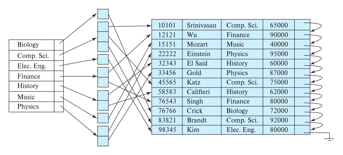 Figure 14.6 · PDF p. 662 · noncandidate key dept_name 위 secondary index가 bucket을 통해 record pointers를 찾는 구조
이 방식은 extra indirection 때문에 index access가 느려질 수 있고, duplicate가 거의 없는 key에 bucket block을 할당하면 space가 낭비된다. 또한 secondary-key order로 file을 sequential scan하려고 하면, 각 record가 서로 다른 disk block에 있을 가능성이 커서 매우 느리다. Secondary indices는 clustering key가 아닌 조건 query를 빠르게 하지만, file modification 때 모든 index를 갱신해야 하므로 write overhead가 크다.
14.2.5 Indices on Multiple Keys
composite search key는 둘 이상의 attributes로 구성된 search key다. Search key는 (a1, ..., an) tuple로 표현되며, ordered index에서는 lexicographic ordering으로 정렬된다. 두 attribute search key에서는 (a1, a2) < (b1, b2) iff a1 < b1이거나 a1 = b1 and a2 < b2다.
예를 들어 takes(course_id, semester, year) index는 특정 course와 semester/year에 등록한 students를 찾는 데 유용하다. Composite key ordered index는 Section 14.6.2에서 보듯 prefix 조건과 여러 형태의 multi-attribute query에도 활용된다.
14.3 B+ -Tree Index Files
index-sequential file organization의 큰 약점은 file이 커지고 insert/delete가 반복되면 lookup과 sequential scan 성능이 떨어진다는 점이다. Reorganization으로 고칠 수는 있지만 자주 reorganize하는 것은 비싸다.
B+ tree index는 insert/delete가 있어도 효율을 유지하는 가장 널리 쓰이는 index structure다. B+ tree는 balanced tree이며 root에서 어떤 leaf까지 가는 모든 path length가 같다. 이 balance property 덕분에 lookup, insertion, deletion의 worst-case가 안정적이다.
Nonleaf node는 root를 제외하면 ceil(n/2)에서 n개의 children을 가진다. Root는 tree가 한 node뿐인 경우를 제외하면 2에서 n개의 children을 가진다. 이런 occupancy 조건 때문에 node가 절반가량 비어 있을 수 있어 space overhead가 생기지만, file reorganization 비용을 피하고 동적인 update에도 성능을 유지하는 이득이 더 크다.
14.3.1 Structure of a B+ -Tree
B+ tree는 multilevel index이지만 단순 multilevel index-sequential file과 다르게 균형 조건과 node occupancy 조건을 유지한다. 우선 search key가 unique하다고 가정하고 구조를 보면, 각 node는 최대 n - 1개의 search-key values K1, K2, ..., K(n-1)와 n개의 pointers P1, P2, ..., Pn을 가진다. Node 안의 search-key values는 sorted order를 유지한다.
Leaf node에서 P1 ... P(n-1)은 각각 search-key value K1 ... K(n-1)를 가진 file record를 가리킨다. 마지막 pointer Pn은 다음 leaf node를 가리키는 데 쓰인다.
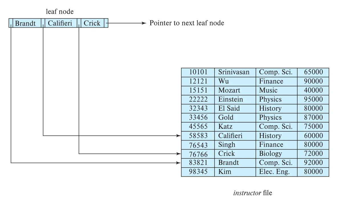 Figure 14.8 · PDF p. 664 · instructor B+ tree index의 leaf node와 다음 leaf로 이어지는 pointer
Leaf node는 최대 n - 1 values를 담고, 최소 ceil((n - 1)/2) values를 담아야 한다. 왼쪽 leaf의 모든 search-key values는 오른쪽 leaf의 모든 search-key values보다 작다. B+ tree가 dense index로 쓰이면 모든 search-key value가 어떤 leaf node에 나타난다.
Leaf들이 search-key order로 linked list처럼 연결되는 것이 B+ tree의 매우 중요한 장점이다. Equality lookup은 root에서 leaf로 내려가고, range query나 sequential scan은 leaf level에서 오른쪽 sibling으로 이동하며 연속적으로 처리할 수 있다.
Nonleaf node는 leaf nodes 위에 놓인 multilevel sparse index처럼 동작한다. Nonleaf node의 모든 pointers는 tree node를 가리키며, pointer 수를 node의 fanout이라고 한다. m개의 pointers를 가진 nonleaf node에서 각 pointer가 담당하는 key range는 다음과 같다.
| Pointer | 담당 search-key range |
|---|---|
P1 | K1보다 작은 values |
Pi, 2 <= i <= m - 1 | K(i-1) <= value < Ki |
Pm | K(m-1)보다 크거나 같은 values |
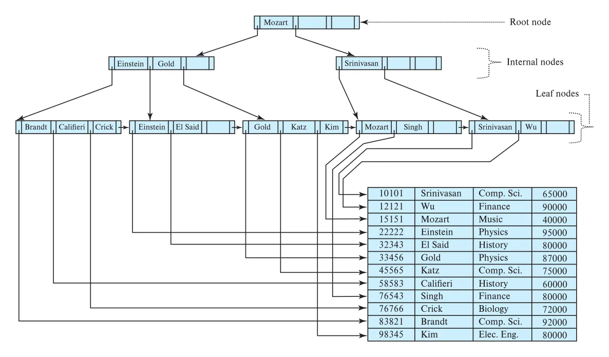 Figure 14.9 · PDF p. 665 · root, internal nodes, leaf nodes로 구성된 instructor B+ tree index
Figure 14.9는 n = 4인 B+ tree다. n이 커지면 fanout이 커지고 height는 낮아진다. 책의 Figure 14.10은 n = 6일 때 같은 instructor file의 tree height가 더 낮아지는 예를 보여 준다. 이 때문에 B+ tree는 binary tree와 달리 disk block 크기에 맞춰 “넓고 낮은(fat and short)” 구조를 택한다.
Nonunique search key는 B+ tree 구현에서 별도 처리가 필요하다. Leaf에 같은 key를 record 수만큼 중복 저장하거나 key마다 pointer bucket을 둘 수 있지만, internal node 중복과 update 복잡도 또는 indirection overhead가 생긴다. 많은 DBMS는 nonunique attribute ai에 index를 만들 때 primary key Ap를 붙여 unique composite search key (ai, Ap)를 내부적으로 사용한다. 예를 들어 instructor.name이 중복될 수 있으면 (name, ID)를 index key로 사용한다.
14.3.2 Queries on B+ -Trees
Equality lookup find(v)는 root에서 시작해 leaf까지 내려간다. 현재 node에서 v <= Ki를 만족하는 가장 작은 i를 찾고, v = Ki이면 Pi+1 쪽으로, v < Ki이면 Pi 쪽으로 내려간다. 그런 i가 없으면 마지막 non-null pointer Pm으로 내려간다. Leaf에 도착한 뒤 leaf 안에 Ki = v가 있으면 Pi가 record pointer이고, 없으면 결과가 없다.
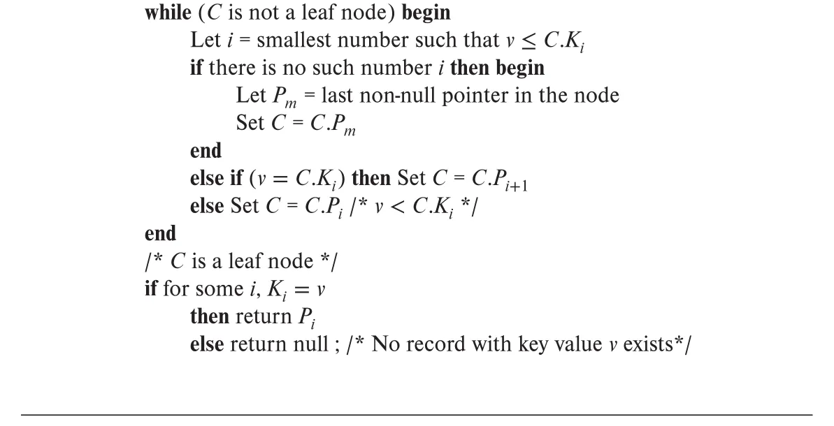 Figure 14.11 · PDF p. 667 · root에서 leaf까지 내려가 search-key value v를 찾는 B+ tree lookup 절차
Range query findRange(lb, ub)는 먼저 lb가 들어갈 leaf까지 내려간 뒤, leaf entries를 오른쪽으로 훑으며 lb <= Ki <= ub인 record pointers를 모은다. 현재 leaf가 끝나면 leaf chain의 next pointer로 다음 leaf로 이동하고, Ki > ub가 되거나 더 이상 leaf가 없으면 멈춘다.
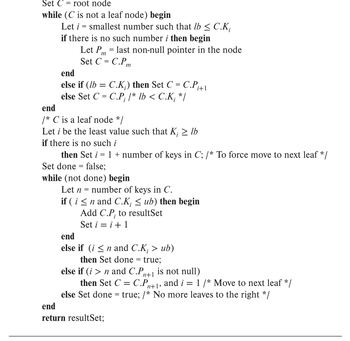 Figure 14.12 · PDF p. 668 · leaf chain을 따라가며 [lb, ub] range의 record pointers를 모으는 B+ tree range query
실제 DBMS는 range query 결과를 한 번에 set으로 만드는 대신 iterator interface를 제공하는 경우가 많다. JDBC ResultSet의 next()처럼 호출할 때마다 leaf-level entry를 한 단계씩 진행하고, 어디까지 읽었는지 상태를 유지한다.
B+ tree lookup cost
B+ tree lookup은 root-to-leaf path 길이에 비례한다. File에 N records가 있고 node fanout이 n이면 path length는 대략 ceil(log_{ceil(n/2)}(N)) 이하로 작다.
보통 node size는 disk block size, 예를 들어 4 KB에 맞춘다. Search-key size가 12 bytes이고 disk pointer가 8 bytes라면 n은 약 200이고, 보수적으로 search-key size를 32 bytes로 잡아도 n은 약 100이다. n = 100, N = 1,000,000이면 lookup은 약 ceil(log_50(1,000,000)) = 4 nodes만 접근한다. Root node는 자주 access되어 buffer에 있을 가능성이 높으므로 실제 disk reads는 더 적을 수 있다.
Binary tree와 B+ tree의 차이는 node 크기와 fanout이다. Binary tree는 node가 작고 pointer가 최대 2개라 thin and tall 구조가 된다. B+ tree는 node 하나가 disk block 크기이고 많은 pointers를 가지므로 fat and short 구조가 되어 disk I/O를 줄인다.
Unique search key의 single-value query는 leaf까지 내려간 뒤 matching record를 fetch하기 위한 random I/O가 추가될 수 있다. Range query는 leaf level에서 consecutive leaf nodes를 읽어 pointers를 모으므로 pointer retrieval은 효율적이지만, 실제 records 접근 비용은 clustering 여부에 따라 크게 달라진다. Secondary index라면 matching records가 서로 다른 blocks에 흩어져 최악의 경우 M random I/Os가 필요할 수 있고, clustered index라면 consecutive blocks에 여러 records가 모여 훨씬 싸다.
Nonunique attribute ai를 (ai, Ap) composite key로 unique하게 만든 경우, ai = v인 모든 tuples는 findRange((v, -infinity), (v, infinity)) 형태로 찾을 수 있다. 즉 unique composite key를 쓰더라도 prefix attribute에 대한 equality/range lookup을 B+ tree range query로 처리할 수 있다.
14.3.3 Updates on B+ -Trees
Relation에 record가 inserted/deleted되면 relation의 indices도 갱신되어야 한다. Record update는 old record deletion과 new record insertion으로 볼 수 있으므로, B+ tree update의 핵심은 insertion과 deletion이다.
Lookup과 달리 insertion/deletion은 node가 너무 커지거나 작아지는 문제를 처리해야 한다. Insert로 leaf 또는 internal node가 capacity를 넘으면 split이 필요하고, delete로 node가 minimum occupancy보다 작아지면 sibling과 coalesce하거나 redistribute해야 한다. 이때 root-to-leaf path length가 모두 같다는 balance property를 유지해야 한다.
14.3.3.1 Insertion
기본 insertion은 먼저 find()와 같은 방식으로 search-key value가 들어갈 leaf node를 찾는다. Leaf에 공간이 있으면 sorted order가 유지되도록 (search-key value, record pointer) entry를 삽입한다.
Leaf에 공간이 없으면 leaf split이 발생한다. 예를 들어 Figure 14.9의 tree에 Adams를 삽입하면 Brandt, Califieri, Crick이 있던 leaf가 overfull이 된다. 일반적으로 기존 n - 1 values와 새 value를 합친 n values를 정렬한 뒤, 앞 ceil(n/2)개는 기존 leaf에, 나머지는 새 leaf에 둔다. 새 leaf의 smallest search-key value와 새 leaf pointer를 parent에 삽입한다.
Parent에 공간이 없으면 internal node split이 parent 쪽으로 전파된다. Figure 14.15는 Lamport 삽입으로 leaf split이 일어나고, 새 separator가 parent에 들어가면서 parent도 split되는 상황을 보여 준다.
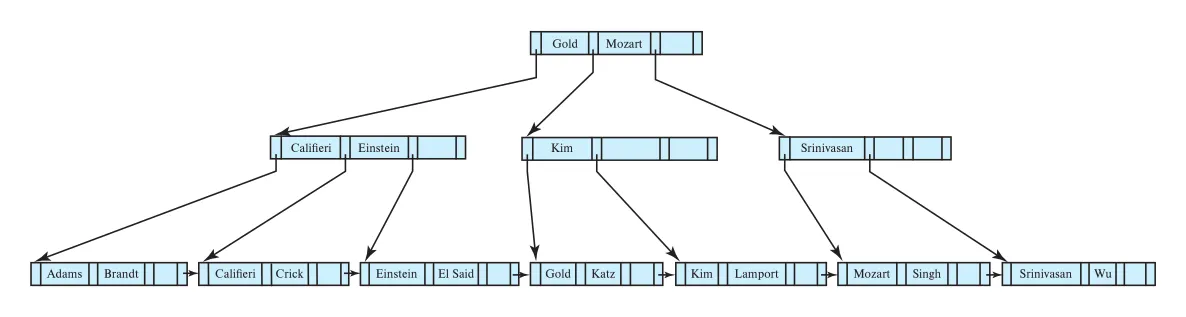 Figure 14.15 · PDF p. 672 · Lamport 삽입 후 leaf split과 parent split이 반영된 B+ tree
Leaf split과 nonleaf split은 separator 처리 방식이 다르다.
| split 대상 | split 후 parent로 올라가는 값 |
|---|---|
| leaf node | 새 right leaf의 smallest key value가 parent에 복사된다. 그 key는 leaf에도 남아 있다. |
| nonleaf node | left/right child pointer들을 나누는 middle separator key가 parent로 올라가며 split된 nonleaf에는 남지 않는다. |
Nonleaf split에서 separator key가 child node에 남지 않는 이유는 nonleaf key가 실제 record pointer를 대표하는 data entry가 아니라 child subtree range를 나누는 boundary 역할이기 때문이다.
Insertion algorithm의 전체 흐름은 다음과 같다.
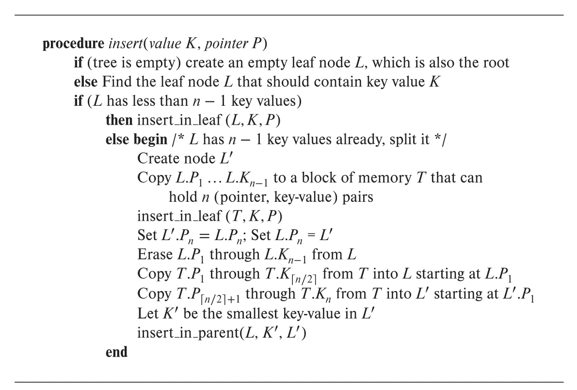 Figure 14.16 · PDF p. 672 · leaf insertion, leaf split, insert-in-parent를 포함한 B+ tree insertion 절차
요약하면 insert(K, P)는 leaf L을 찾고, 공간이 있으면 insert in leaf(L, K, P)를 수행한다. 공간이 없으면 temporary area T에서 기존 entries와 새 entry를 정렬한 뒤 L과 새 leaf L'로 나누고, L'의 smallest key K'를 insert in parent(L, K', L')로 parent에 반영한다. Parent split도 재귀적으로 같은 방식으로 처리되며, root가 split되면 새 root가 만들어져 tree depth가 1 증가한다.
14.3.3.2 Deletion
Deletion은 먼저 lookup으로 (K, P)가 들어 있는 leaf node를 찾고 entry를 제거한다. 제거 후 leaf가 minimum number of values 이상을 유지하면 끝난다. Underfull이 되면 adjacent sibling과 합칠 수 있는지 먼저 확인한다.
Deletion에서 가능한 복구 방식은 두 가지다.
| 방식 | 조건 | 동작 |
|---|---|---|
coalesce 또는 merge | underfull node와 sibling의 entries가 한 node에 들어갈 수 있음 | 두 node를 하나로 합치고, parent에서 삭제된 node를 가리키던 entry를 제거한다. |
redistribution | 두 node를 합치면 capacity를 넘음 | sibling에서 entry/pointer를 빌려 양쪽 occupancy를 맞추고, parent separator key를 갱신한다. |
Leaf merge는 leaf-level entries와 next-leaf pointer를 조정한다. Nonleaf merge는 parent의 separator key가 merged node 안으로 내려올 수 있다. Redistribution에서는 sibling에서 이동한 entry에 맞춰 parent의 separator key도 바뀐다. 즉 deletion은 leaf에서 끝나지 않고 parent separator를 수정하거나 parent deletion을 재귀적으로 유발할 수 있다.
Figure 14.20은 Gold deletion 이후 underfull leaf merge가 parent underfull로 이어지고, 결국 root가 child 하나만 남게 되어 root가 삭제되고 그 sole child가 새 root가 되는 상황을 보여 준다. 이때 B+ tree의 depth가 1 감소한다.
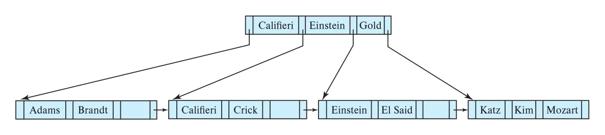 Figure 14.20 · PDF p. 676 · Gold 삭제 후 merge가 root까지 전파되어 tree depth가 줄어든 B+ tree
Deletion 뒤에는 leaf level에는 없는 key가 nonleaf node에 남을 수 있다. 예를 들어 Figure 14.20에서 Gold는 leaf level에서 삭제되었지만 nonleaf separator로 남아 있다. 이는 nonleaf key가 record 자체가 아니라 subtree boundary를 표현하기 때문이다.
Deletion algorithm은 다음처럼 underfull 처리와 root shrink를 포함한다.
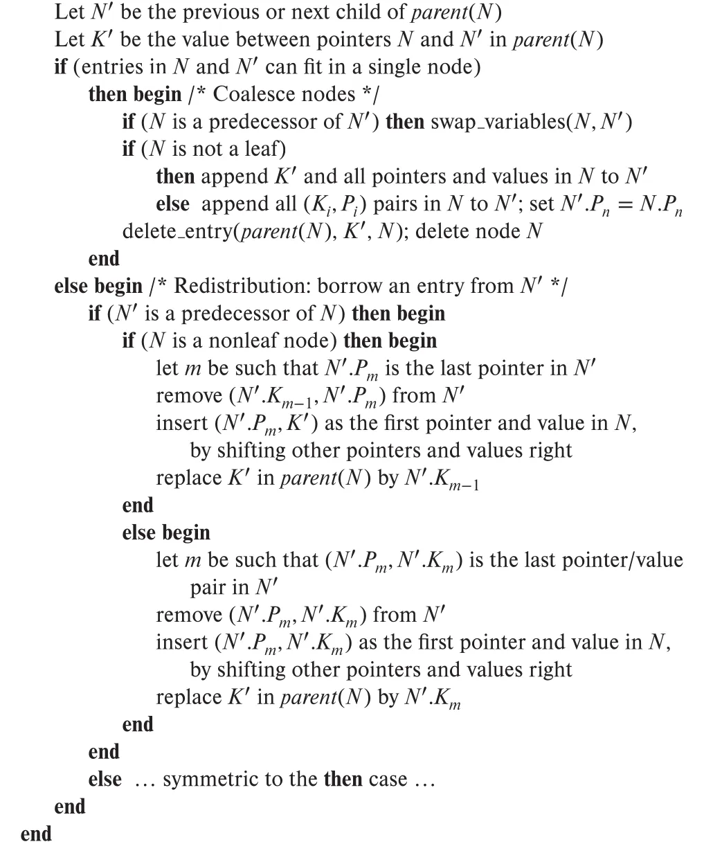 Figure 14.21 · PDF p. 677 · coalesce, redistribution, root shrink를 포함한 B+ tree deletion 절차
Pseudo-code의 “too few pointers/values”는 node 종류에 따라 다르다. Nonleaf node는 ceil(n/2)보다 적은 pointers면 underfull이고, leaf node는 ceil((n - 1)/2)보다 적은 values면 underfull이다. Algorithm은 adjacent node에서 한 entry를 borrow하는 redistribution을 보이지만, 두 nodes의 entries를 균등하게 repartition하는 방식도 가능하다.
14.3.4 Complexity of B+ -Tree Updates
B+ tree insertion/deletion은 알고리즘상 복잡해 보이지만 I/O 관점에서는 낮은 비용을 유지한다. Worst case insertion은 root-to-leaf path를 따라 split이 전파될 수 있으므로 log_{ceil(n/2)}(N)에 비례한다. Deletion도 unique search key 기준으로 같은 order의 worst-case I/O를 가진다.
실제로는 worst case보다 훨씬 적은 I/O가 발생한다. Fanout이 100이면 leaf parent는 leaf보다 100배 자주 access되므로 buffer에 있을 가능성이 높고, 전체 nonleaf node 수는 leaf node 수의 약 1/100보다 조금 많은 정도다. 자주 쓰이는 B+ tree라면 대부분의 nonleaf nodes가 database buffer에 올라와 있어 lookup은 보통 1-2번의 disk I/O로 끝난다.
Update에서도 split은 드물다. Fanout 100 기준으로 insert ordering에 따라 대략 50-100번 insert 중 1번 정도만 node split이 발생할 수 있다. Random order로 entries가 삽입되면 nodes는 평균적으로 2/3 이상 차는 경향이 있고, sorted order로 삽입되면 split 패턴 때문에 nodes가 절반 정도만 차는 경향이 있다.
14.3.5 Nonunique Search Keys
Nonunique search key를 처리하는 가장 흔한 방식은 원래 search key에 uniquifier attribute를 붙여 unique composite search key를 만드는 것이다. Uniquifier attribute는 record-id, primary key, 또는 같은 search-key value group 안에서 unique한 attribute일 수 있다. 원래 search key만으로 lookup할 때는 range search를 사용하거나, uniquifier attribute를 비교에서 무시하는 findRange 변형을 쓸 수 있다.
Duplicate search keys를 B+ tree 자체에서 직접 지원할 수도 있지만 trade-off가 있다.
| 방식 | 장점 | 문제 |
|---|---|---|
| key value를 한 번만 저장하고 bucket/list에 record pointers 저장 | key 저장 공간 절약 | variable-size bucket 처리, bucket overflow, separate bucket block I/O 발생 가능 |
| record마다 search key value를 반복 저장 | leaf split을 일반 방식으로 처리 가능 | internal node split/search 복잡도 증가, key 중복으로 space overhead 증가 |
| uniquifier를 붙인 unique composite key | lookup/insert/delete를 기존 B+ tree 방식으로 유지 | key size가 커질 수 있고 DBMS가 내부 attribute를 추가해야 함 |
두 duplicate-key 방식의 큰 약점은 deletion이다. 어떤 search-key value가 매우 많이 반복될 때 특정 record를 삭제하려면 같은 key entries를 여러 leaf nodes에 걸쳐 찾아야 할 수 있어 worst-case deletion이 record 수에 선형적으로 가까워질 수 있다. 반면 unique composite key 방식은 삭제할 record에서 composite key를 계산해 root-to-leaf traversal 한 번으로 정확한 leaf entry를 찾을 수 있으므로 logarithmic cost를 유지한다.
그래서 대부분의 database B+ tree implementation은 내부적으로 record-id나 다른 attributes를 자동으로 추가해 nonunique search key를 unique하게 만든다.
14.4 B+ -Tree Extensions
이 절은 B+ tree를 단순 index structure에서 실제 storage/file organization, secondary index, string key, bulk loading, flash/main-memory 환경으로 확장할 때 생기는 문제를 다룬다.
14.4.1 B+ -Tree File Organization
B+ tree file organization은 leaf node가 record pointer가 아니라 실제 records를 저장하는 방식이다. 즉 B+ tree를 index로만 쓰는 것이 아니라 file records 자체의 organizer로 사용한다.
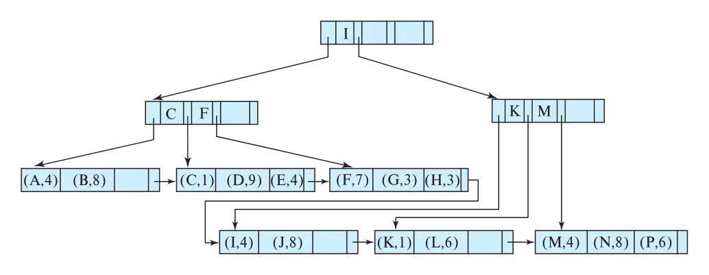 Figure 14.22 · PDF p. 680 · leaf level에 actual records를 저장하는 B+ tree file organization
Index-sequential file은 file이 성장하면서 overflow blocks가 늘고 physical order가 깨져 성능이 떨어진다. B+ tree file organization은 records가 들어 있는 leaf blocks도 B+ tree update 규칙으로 split/merge하므로 lookup degradation을 줄인다.
Record가 v라는 key로 삽입되면, system은 v 이하의 가장 큰 key가 있는 leaf block을 찾아 그 block에 record를 넣는다. 공간이 없으면 block을 split하고 records를 B+ tree key order로 재분배한다. Deletion으로 block이 half full보다 작아지면 adjacent block과 redistribute 또는 merge한다.
File organization에서는 key/pointer보다 actual record space가 훨씬 크므로 space utilization이 중요하다. 그래서 split/merge 때 단순히 두 siblings만 보는 대신 더 많은 adjacent siblings를 포함해 재분배할 수 있다. 세 nodes를 함께 고려하면 split 후 각 node를 약 2/3 이상 차게 만들 수 있다. 더 많은 siblings를 쓰면 utilization은 좋아지지만 update cost가 커진다.
Leaf nodes가 tree에서 adjacent하더라도 disk에서는 점점 흩어질 수 있다. 새로 만든 file은 leaf-contiguous blocks를 disk-contiguous하게 배치할 수 있지만, insert/delete가 반복되면 sequentiality가 깨진다. 이때 sequential scan 성능을 회복하려면 index rebuild가 필요할 수 있다.
B+ tree file organization은 SQL clob, blob 같은 large object에도 쓸 수 있다. Large object를 smaller records sequence로 쪼개고, record number 또는 byte offset을 search key로 사용하면 object의 range access를 B+ tree로 처리할 수 있다.
14.4.2 Secondary Indices and Record Relocation
B+ tree file organization에서는 record 자체가 leaf split 때문에 다른 leaf block으로 이동할 수 있다. Record value가 바뀌지 않았더라도 physical location이 바뀌면, record pointer를 저장한 모든 secondary indices를 갱신해야 한다. Leaf split 하나가 많은 records를 이동시키고, 각 record가 여러 secondary index에 흩어져 있으면 수십-수백 I/O가 필요할 수 있다.
널리 쓰이는 해결책은 secondary index에 physical record pointer 대신 primary-index search-key value를 저장하는 것이다. 예를 들어 instructor.ID가 primary index라면, dept_name secondary index는 record pointer 대신 해당 instructor의 ID values를 저장한다.
이 방식은 record relocation 때 secondary index를 고치지 않아도 되는 장점이 있다. 대신 secondary index lookup은 두 단계가 된다.
- Secondary index로 primary-index search-key value를 찾는다.
- Primary index로 actual record를 찾는다.
즉 update/reorganization 비용을 줄이는 대신 secondary index access cost를 늘리는 trade-off다.
14.4.3 Indexing Strings
String-valued attribute에 B+ tree index를 만들면 두 문제가 생긴다. 첫째, strings는 variable length다. 둘째, strings가 길면 node fanout이 낮아져 tree height가 커진다.
Variable-length search keys에서는 full node 판단을 entry 개수가 아니라 node space 사용량으로 해야 한다. Split/merge/redistribution도 maximum entry count가 아니라 공간 사용 fraction을 기준으로 판단한다.
Fanout을 높이는 대표 기법은 prefix compression이다. Nonleaf node에 full search-key value를 저장하지 않고, 두 subtrees의 key ranges를 구분하기에 충분한 prefix만 저장한다. 예를 들어 Silas와 Silver 사이를 구분하려면 Silberschatz 전체가 아니라 Silb 같은 prefix만 저장해도 될 수 있다.
14.4.4 Bulk Loading of B+ -Tree Indices
Large relation 위에 B+ tree를 처음 만들 때 tuple-at-a-time insertion은 매우 비쌀 수 있다. Relation이 memory보다 크고 index도 memory보다 크면, random order로 leaf nodes를 계속 fetch/write-back해야 하므로 entry 하나마다 random read와 random write가 발생할 수 있다.
bulk loading은 많은 index entries를 한 번에 삽입하는 방법이다. 효율적인 방식은 다음 순서다.
- Relation을 scan해 temporary file에 index entries를 만든다.
- Temporary file을 index search key로 sort한다.
- Sorted entries를 순서대로 scan하면서 B+ tree에 삽입하거나, empty tree라면 bottom-up으로 구성한다.
Sorted order로 삽입하면 같은 leaf node에 들어갈 entries가 연속해서 나타나므로 leaf node를 한 번만 쓰면 된다. Empty B+ tree에서는 bottom-up construction이 더 빠르다. Sorted entries를 leaf blocks로 채우고, 각 leaf block의 minimum value와 pointer로 next level을 만들며, root가 생길 때까지 반복한다.
실무적으로는 대량 tuple을 기존 relation에 넣을 때 primary key index 외의 indices를 drop한 뒤 load가 끝나면 다시 create하는 전략이 bulk-loading benefit을 얻을 수 있다.
14.4.5 B-Tree Index Files
B-tree와 B+ tree는 이름이 비슷하지만 이 책에서는 구분한다. B+ tree에서는 모든 search-key values가 leaf에 있고, 일부 separator keys가 nonleaf에도 중복 저장된다. B-tree는 unique search-key value를 한 번만 저장하려고 하며, nonleaf에 있는 key는 leaf에 다시 나타나지 않는다.
Figure 14.24는 B-tree node에서 nonleaf node가 tree pointers Pi뿐 아니라 해당 key의 record/bucket pointer Bi도 함께 가져야 함을 보여 준다.
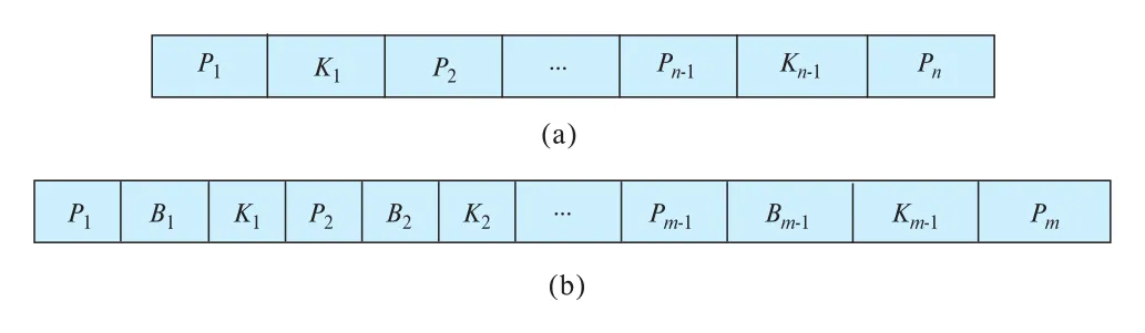 Figure 14.24 · PDF p. 685 · B-tree leaf node와 nonleaf node의 pointer/key 배치
B-tree의 장단점은 다음과 같다.
| 구분 | B-tree | B+ tree |
|---|---|---|
| key 중복 | unique key를 한 번만 저장 | leaf key와 nonleaf separator가 중복될 수 있음 |
| nonleaf payload | record/bucket pointer Bi도 필요 | child pointer와 separator key 중심 |
| fanout | nonleaf payload 때문에 더 작을 수 있음 | 더 큰 fanout 가능 |
| lookup | 어떤 key는 leaf 전에 찾을 수 있음 | 항상 leaf까지 내려감 |
| range/sequential scan | leaf-only structure보다 불리 | leaf chain으로 효율적 |
| deletion | nonleaf key 삭제 가능성 때문에 복잡 | 삭제 entry는 leaf에 있음 |
B-tree의 space 이점은 큰 index에서는 보통 미미하고, fanout 감소와 deletion 복잡도가 단점이 된다. 실제 database system은 대부분 B+ tree를 사용하며, industry 문서에서 B-tree라고 부르는 구조가 실제로는 B+ tree인 경우도 많다.
14.4.6 Indexing on Flash Storage
SSD/flash storage에서도 standard B+ tree는 계속 사용할 수 있다. Random page read가 magnetic disk의 5-10 ms보다 훨씬 빠른 20-100 microseconds 수준이어서 lookup 성능은 크게 좋아진다.
하지만 flash는 physical in-place update를 허용하지 않는다. Logical update도 실제로는 새 flash page에 copy+write하고, old page는 나중에 block erase로 정리한다. Page write는 빠르지만 erase는 multiple pages를 포함한 block 단위로 일어나며 2-5 ms가 걸릴 수 있다.
따라서 flash에 맞는 B+ tree node size는 magnetic disk보다 작아지는 경향이 있다. Flash page에 node size를 맞추면 update 때 여러 page writes를 줄일 수 있다. Smaller nodes는 tree height를 높일 수 있지만 flash random reads가 매우 빠르므로 read 성능 영향은 상대적으로 작다.
SSD에서도 bulk loading은 여전히 유리하다. Bottom-up construction은 tuple-at-a-time insertion보다 page writes 수를 줄이고, flash의 erase cost를 줄이는 데 도움이 된다. Flash write cost를 줄이는 대안으로 internal node buffer에 updates를 임시로 모았다가 lazy하게 아래로 내리는 방식과, multiple trees를 만들고 merge하는 log-structured merge tree (LSM tree) 계열이 있다. 이들은 Section 14.8과 Chapter 24로 이어진다.
14.4.7 Indexing in Main Memory
Main-memory data에도 B+ tree를 그대로 사용할 수 있지만, optimization 기준은 disk I/O가 아니라 space와 CPU cache miss다.
Memory는 disk보다 비싸므로 in-memory B+ tree는 storage utilization을 높이는 기법이 중요하다. 또한 disk와 달리 multiple pointer traversal이 큰 I/O 비용을 일으키지는 않으므로 tree가 상대적으로 깊어도 받아들일 수 있다.
반면 cache memory와 main memory 사이의 latency 차이는 중요하다. Cache hit는 1-2 ns 수준이지만 cache miss는 main memory read 때문에 50-100 ns delay가 날 수 있다. B+ tree node를 cache line, 보통 64 bytes 정도에 맞게 작게 만들면 node traversal마다 발생하는 cache misses를 줄일 수 있다.
Disk와 memory를 모두 고려해야 하는 system에서는 disk access를 위해 large B+ tree node를 쓰되, node 내부를 하나의 큰 array로 보지 않고 cache-line-sized small nodes로 된 작은 tree처럼 구성할 수 있다. 이렇게 하면 disk block fanout과 cache locality를 동시에 어느 정도 얻는다.
14.5 Hash Indices
hash index는 search-key value에 hash function을 적용해 bucket을 찾는 index다. Main memory hash index는 join processing에서 transient structure로 만들어질 수도 있고, main-memory database의 permanent structure로 쓰일 수도 있다. Disk-based hash file organization은 존재하지만 널리 쓰이지는 않는다.
bucket은 one or more records 또는 index entries를 저장하는 단위다. In-memory hash index에서는 bucket이 linked list head pointer일 수 있고, disk-based hash index에서는 bucket이 disk blocks의 linked list일 수 있다.
Formal하게 search-key values 집합을 K, bucket addresses 집합을 B라고 하면, hash function h는 K -> B mapping이다. Insert할 때는 h(Ki)를 계산해 해당 bucket에 index entry를 넣는다.
책이 설명하는 대표 방식은 overflow chaining이다. 같은 bucket에 여러 entries가 들어가면 linked list로 연결한다. 이 방식은 closed addressing 또는 closed hashing이라고도 부른다. open addressing은 delete를 효율적으로 지원하지 않아 database indexing에는 일반적으로 적합하지 않다.
Hash index의 강점과 약점은 뚜렷하다.
| access | hash index의 성격 |
|---|---|
| equality query | h(Ki)로 bucket을 바로 찾고 bucket 안 entries만 비교하므로 효율적 |
| range query | hash value가 key order를 보존하지 않으므로 l <= v <= u를 효율적으로 처리하지 못함 |
| deletion | h(Ki) bucket을 찾아 linked list에서 해당 record를 제거 |
Disk-based hash index에서 bucket이 가득 차면 bucket overflow가 발생한다. DBMS는 해당 bucket에 overflow bucket을 할당하고, overflow buckets를 linked list로 연결한다.
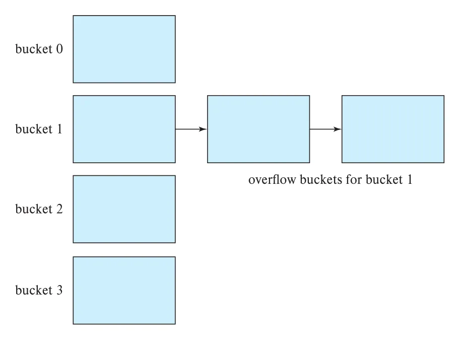 Figure 14.25 · PDF p. 689 · bucket overflow가 발생한 disk-based hash structure의 overflow chaining
Overflow는 bucket 수가 records 수에 비해 부족하거나, hash function이 keys를 uniform/random하게 분배하지 못하거나, 같은 search-key value가 많이 반복되어 skew가 생길 때 발생한다. Overflow 가능성을 줄이기 위해 bucket 수는 보통 (nr / fr) * (1 + d)처럼 약간 여유 있게 잡는다. 여기서 nr은 record 수, fr은 bucket당 record 수, d는 fudge factor이며 보통 0.2 정도를 둘 수 있다.
Bucket 수를 index 생성 시 고정하는 방식을 static hashing이라고 한다. Records가 예상보다 많이 늘면 overflow chain이 길어져 lookup이 느려진다. 이때 index를 더 많은 buckets로 rebuild할 수 있지만 large relation에서는 오래 걸리고 service disruption이 생긴다. Bucket 수를 incremental하게 늘리는 방식은 dynamic hashing techniques이고, linear hashing, extendable hashing이 대표적이며 Chapter 24.5에서 더 깊게 다룬다.
14.6 Multiple-Key Access
지금까지는 query가 하나의 index를 사용한다고 보았지만, 실제 query는 여러 predicates를 동시에 가진다. 이때 여러 single-key indices를 조합하거나 composite search key index를 사용할 수 있다.
14.6.1 Using Multiple Single-Key Indices
예를 들어 instructor에 dept_name index와 salary index가 있고 다음 query를 실행한다고 하자.
select ID
from instructor
where dept_name = 'Finance' and salary = 80000;
가능한 전략은 세 가지다.
| 전략 | 동작 | 장단점 |
|---|---|---|
dept_name index만 사용 | Finance records를 찾고 salary를 검사 | dept_name selectivity가 높으면 좋다. |
salary index만 사용 | salary 80000 records를 찾고 dept_name을 검사 | salary selectivity가 높으면 좋다. |
| 두 index 사용 | 각 index에서 record pointers를 얻고 intersection | 두 조건을 모두 활용하지만 pointer set이 크면 비쌀 수 있다. |
세 번째 전략은 multiple indices를 실제로 활용하지만, 각 조건의 result set은 크고 intersection만 작으면 많은 pointers를 scan해서 작은 결과를 만드는 비효율이 생긴다. 이런 intersection 연산은 Section 14.9의 bitmap index가 빠르게 처리할 수 있다.
14.6.2 Indices on Multiple Keys
대안은 composite search key (dept_name, salary) 위에 ordered B+ tree index를 만드는 것이다. 이 index는 dept_name = 'Finance' and salary = 80000 같은 equality 조건을 빠르게 처리한다.
Composite ordered index는 첫 attribute에 equality가 있고 두 번째 attribute에 range가 있는 query도 잘 처리한다.
select ID
from instructor
where dept_name = 'Finance' and salary < 80000;
위 조건은 (Finance, -infinity)부터 (Finance, 80000)까지의 composite-key range query로 처리할 수 있다. dept_name = 'Finance'만 있는 query도 (Finance, -infinity)부터 (Finance, +infinity)까지의 range로 볼 수 있다.
하지만 첫 attribute에 range/comparison이 걸리면 문제가 달라진다.
select ID
from instructor
where dept_name < 'Finance' and salary < 80000;
이 조건은 (dept_name, salary) 전체 search key의 단일 contiguous range로 잘 대응되지 않는다. 각 dept_name < Finance 값마다 salary 조건을 따로 보아야 하고, records가 서로 다른 disk blocks에 흩어질 수 있다. 일반적인 multi-dimensional range query에는 bitmap index나 Section 14.10.1의 R-tree 같은 구조가 더 적합할 수 있다.
14.6.3 Covering Indices
covering index는 search-key attributes 외의 일부 attribute values를 record pointer와 함께 저장하는 index다. 특히 secondary index에서 유용하다. Index 안에 query가 필요한 attributes가 모두 있으면 actual record를 fetch하지 않고 index만으로 query를 답할 수 있다.
예를 들어 instructor.ID에 nonclustering index가 있고 index entry에 salary도 함께 저장하면, ID로 찾고 salary만 필요한 query는 instructor record를 읽지 않아도 된다. (ID, salary) composite key index를 만드는 것과 비슷한 효과가 있지만, covering index는 salary를 search key 일부로 쓰지 않으므로 nonleaf node fanout을 덜 줄이고 tree height 증가를 피할 수 있다.
14.7 Creation of Indices
SQL standard는 index creation syntax를 직접 지정하지 않지만, 대부분의 DBMS는 다음 형태를 지원한다.
create index <index-name> on <relation-name> (<attribute-list>);
drop index <index-name>;attribute-list는 index search key를 구성하는 attributes다. Candidate key임을 index로 선언하려면 보통 create unique index를 사용한다. 여러 index type을 지원하는 DBMS는 index creation command에서 B+ tree, hash, bitmap 등 index type을 지정할 수 있다.
Index를 만들 후보는 selection condition 또는 join condition에 자주 등장하는 attributes다. 예를 들어 takes.ID = 12345 조건이 많다면 takes(ID) index가 있으면 몇 번의 I/O로 pointer를 얻고, 실제 record도 학생 한 명의 수강 records 정도만 가져오면 된다. Index가 없으면 takes 전체를 scan해야 한다.
하지만 index는 update cost를 만든다. Underlying relation이 update될 때 affected indices도 모두 update해야 한다. 따라서 “query 하나가 빨라진다”만 보고 index를 마구 만들면 write/update workload가 느려질 수 있다.
원문은 application testing에서 index 필요성이 과소평가될 수 있음을 강조한다. 단일 query가 1초라면 테스트 중에는 충분히 빨라 보일 수 있지만, 한 시간에 1000 students가 각각 10 queries를 실행하면 총 query execution time이 10,000초가 되어 system이 느려질 수 있다. Index로 query가 10 ms로 줄면 같은 workload의 총 시간이 100초 수준으로 내려간다. 즉 index design은 single-query latency뿐 아니라 workload concurrency와 frequency를 함께 봐야 한다.
Primary key를 선언하면 대부분의 DBMS는 자동으로 primary-key index를 만든다. Insert 시 duplicate primary-key value가 있는지 전체 relation scan 없이 확인하기 위해서다. Foreign-key attributes에도 index를 두는 것이 좋은 경우가 많다. 대부분의 join은 foreign key와 primary key 사이에서 일어나며, referenced table에 selective condition이 있으면 foreign-key side tuples를 빠르게 찾는 것이 중요하다.
DBMS는 query/update frequency를 추적해 index 생성을 추천하는 index tuning wizard 또는 advisor를 제공하기도 한다. 일부 cloud database는 반복 relation scan을 피하기 위해 자동으로 index를 만들기도 한다.
14.8 Write-Optimized Index Structures
B+ tree는 lookup과 일반 update에는 좋지만, memory에 다 들어가지 않는 큰 index에서 random writes/inserts가 매우 많으면 약해진다. Insert order가 index sort order와 맞지 않으면 각 insert가 다른 leaf page를 건드리고, leaf pages 수가 buffer보다 훨씬 많으면 insert마다 random read와 write가 필요해진다.
Magnetic disk에서는 seek 때문에 per-disk write throughput이 크게 제한된다. SSD에서는 random I/O가 빠르지만 page write가 결국 erase cost를 유발하므로 random write-heavy workload에는 여전히 부담이 있다. 그래서 write-optimized index structures가 등장한다. 대표적으로 log-structured merge tree (LSM tree)와 buffer tree가 있다.
14.8.1 LSM Trees
LSM tree는 여러 B+ trees로 구성된다. 맨 위에는 in-memory tree L0가 있고, disk에는 L1, L2, ..., Lk가 있다.
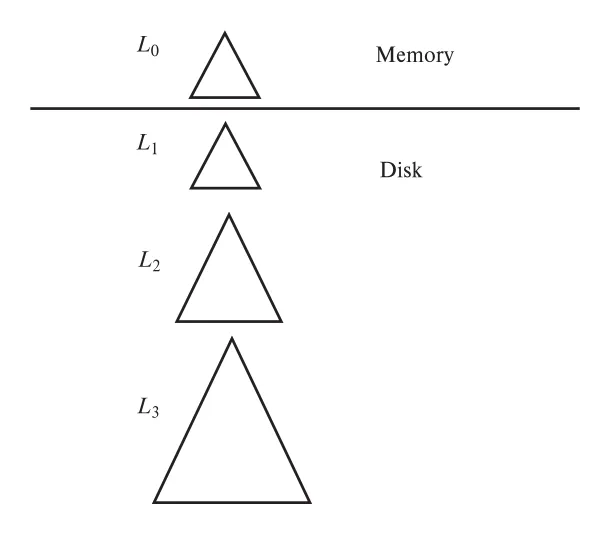 Figure 14.26 · PDF p. 695 · memory의 L0와 disk의 L1-L3로 구성된 three-level LSM tree
Insert는 먼저 memory의 L0 B+ tree에 들어간다. L0가 할당된 memory를 채우면, L0의 leaf level을 search-key order로 scan해 disk tree L1과 merge한다. L1이 비어 있으면 L0 전체를 disk로 써서 L1을 만들고, L1이 이미 있으면 old L1 leaf entries와 L0 entries를 sorted order로 merge해 새 B+ tree를 bottom-up으로 만든 뒤 old L1을 대체한다.
LSM merge의 장점은 다음과 같다.
| 장점 | 이유 |
|---|---|
| sequential I/O | leaf entries를 sorted order로 scan/merge하므로 random leaf update를 피한다. |
| full leaves | 새 tree를 bottom-up으로 만들기 때문에 leaf pages가 꽉 찬다. |
| no in-place update | old tree를 갱신하지 않고 새 tree를 만들어 교체한다. SSD/append-only storage와 잘 맞는다. |
단점은 merge 때 old tree 전체를 복사할 수 있다는 점이다. 이를 줄이는 방법은 두 가지다.
| 변형 | 핵심 아이디어 | trade-off |
|---|---|---|
| leveled LSM | Li+1의 max size를 Li보다 k배 크게 하여 level 수를 log_k(I/M)로 제한 | 각 level에서 record가 여러 번 rewrite될 수 있음 |
stepped-merge index | 각 disk level에 여러 trees를 허용하고, b개가 쌓이면 next level로 merge | insert cost 감소, lookup은 여러 trees를 봐야 함 |
Stepped-merge는 query cost가 커질 수 있으므로 Bloom filter로 어떤 tree에 search key가 없는지 빠르게 판단한다. Bloom filter는 작은 space로 negative lookup을 효율적으로 줄인다.
Deletes는 실제 entry를 찾아 즉시 삭제하지 않고 deletion entry를 insert하는 방식으로 처리한다. Lookup은 normal entry와 deletion entry를 함께 보고 deletion entry가 있으면 해당 entry를 결과에서 제거한다. Merge 때 matching original entry와 deletion entry가 만나면 둘 다 버린다. Updates도 update entry를 insert하고, lookup/merge 때 최신 value를 반영하는 방식으로 처리할 수 있다.
LSM tree는 magnetic disk의 write/seek overhead를 줄이기 위해 고안되었지만, SSD에서도 in-place update를 피하고 write count를 줄인다는 점에서 유리하다. Append-only distributed file system 위의 BigTable, HBase 계열과 BigData storage systems에서 널리 쓰이는 이유도 여기에 있다.
14.8.2 Buffer Tree
buffer tree는 각 internal node에 buffer를 붙인 search tree다. Insert를 leaf까지 즉시 내려보내지 않고 root buffer에 먼저 쌓아 두었다가, buffer가 차면 child nodes로 batch push한다.
 Figure 14.27 · PDF p. 698 · internal node에 search pointers/keys와 별도 buffer를 함께 둔 buffer tree
Insert는 root buffer에 들어간다. Buffer가 가득 차면 buffer records를 search key로 sort하고, 각 child로 내려갈 records를 한꺼번에 push한다. Child가 internal node면 child buffer에 추가하고, child가 leaf면 일반 B+ tree 방식으로 leaf에 삽입한다. Leaf가 overfull이면 B+ tree split이 일어난다. Internal node split 시에는 buffer entries도 key ranges에 따라 나누어야 한다.
Lookup은 일반 B+ tree처럼 leaf까지 내려가되, 지나가는 internal nodes의 buffer도 검사해야 한다. Range lookup은 접근하는 leaf nodes 위의 internal-node buffers도 함께 검사해야 한다.
Buffer tree의 핵심 이득은 amortization이다. Internal buffer가 child 수의 k배 records를 담는다면, push-down 시 평균적으로 child마다 k records가 한 번에 내려간다. Child node를 읽고 쓰는 비용이 k records에 나뉘므로 per-insert I/O cost가 줄어든다.
Buffer tree와 LSM tree의 trade-off는 다음과 같다.
| 구조 | read cost | write pattern | 적합한 저장장치/상황 |
|---|---|---|---|
| LSM tree | 여러 trees를 찾아야 해 lookup cost가 커질 수 있음 | sequential I/O 중심 | magnetic disk, append-only/distributed storage, write-heavy workload |
| buffer tree | LSM보다 read가 빠른 편 | random I/O가 포함됨 | SSD처럼 random I/O가 싼 환경, write 수 자체를 줄이고 싶은 경우 |
Buffer tree의 아이디어는 B+ tree에만 한정되지 않는다. Internal node buffer를 붙여 writes를 batch 처리하는 방식은 R-tree 같은 spatial index의 bulk loading에도 응용될 수 있다.
14.9 Bitmap Indices
bitmap index는 각각 single key에 대해 만들어지지만, multiple-key query를 bit operation으로 빠르게 처리하기 위한 specialized index다. Relation records는 0부터 sequentially numbering되어 있어야 하고, record number n으로 해당 record를 쉽게 찾을 수 있어야 한다. Fixed-size records가 consecutive file blocks에 배치된 경우 record number를 block number와 block 내부 record number로 쉽게 변환할 수 있다.
Bitmap index는 attribute가 가질 수 있는 각 value마다 하나의 bitmap을 둔다. Relation에 records가 N개 있으면 각 bitmap은 N bits를 가진다. Attribute A의 value vj에 대한 bitmap에서 i번째 bit는 record i의 A value가 vj이면 1, 아니면 0이다.
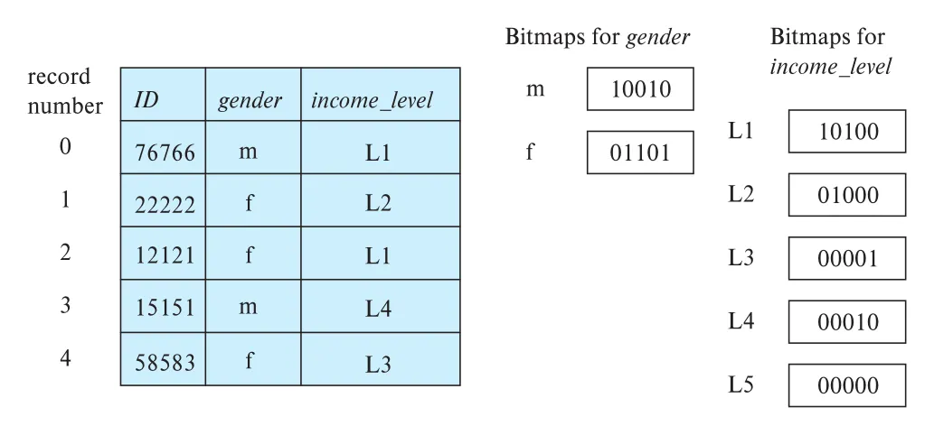 Figure 14.28 · PDF p. 700 · gender와 income_level에 대한 bitmap indices와 bit vectors
Bitmap index는 단일 low-cardinality selection만 빠르게 하지는 못할 수 있다. 예를 들어 gender가 m/f 두 값뿐이면 특정 gender records가 relation의 큰 부분을 차지해 결국 거의 모든 blocks를 읽을 수 있다.
Bitmap의 힘은 multiple predicates를 결합할 때 나온다. 예를 들어 gender = 'f' and income_level = 'L2'는 gender=f bitmap과 income_level=L2 bitmap의 logical AND로 처리한다.
gender = f        01101
income_level=L2  01000
AND              01000
AND 결과에서 1인 positions만 actual records로 fetch하면 된다. Conditions가 여러 개일수록 satisfying fraction이 작아질 가능성이 높아 bitmap intersection 이득이 커진다. 반대로 결과 fraction이 크면 relation 전체 scan이 더 쌀 수 있다.
Bitmap indices는 data warehouse/analytics처럼 low-cardinality 또는 bucketized attribute가 많고, 여러 조건을 조합하는 query가 많은 환경에서 유용하다. Aggregate operation, bitmap compression, B+ tree와 bitmap의 hybrid 구조는 Chapter 24.3에서 더 깊게 다룬다.
14.10 Indexing of Spatial and Temporal Data
전통적인 hash index와 B+ tree는 1차원 search key 또는 lexicographic order에 강하지만, 2차원 이상 spatial data나 time interval을 가진 temporal data에는 성능이 나쁠 수 있다. Spatial query는 area, distance, nearest neighbor처럼 단일 sorted order로 잘 표현되지 않는 조건을 다룬다.
14.10.1 Indexing of Spatial Data
spatial data는 2차원 이상의 point 또는 region을 나타내는 data다. 예를 들어 restaurant location은 (latitude, longitude) point이고, farm/lake의 spatial extent는 여러 corner points로 정의된 polygon일 수 있다.
Spatial data에서 자주 나오는 query는 다음과 같다.
| query type | 예 | 일반 B+ tree의 한계 |
|---|---|---|
| exact point query | 정확히 특정 (latitude, longitude)에 있는 restaurant 찾기 | composite key B+ tree로 처리 가능 |
| spatial range query | 사용자 위치 반경 500m 안의 restaurants 찾기 | lexicographic order와 circular/rectangular region이 잘 맞지 않음 |
| rectangular range query | 관심 rectangular region 안의 objects 찾기 | 한 dimension range만으로 충분하지 않음 |
| nearest neighbor query | 특정 위치에서 가장 가까운 restaurant 찾기 | sorted key order 하나로 거리 최소화를 표현하기 어려움 |
k-d tree는 multidimensional points를 index하기 위한 초기 구조 중 하나다. 각 level에서 하나의 dimension을 기준으로 space를 둘로 나누고, 다음 level에서는 다른 dimension을 기준으로 나누며 dimensions를 순환한다. 각 node의 partition은 subtree에 있는 points가 양쪽에 거의 절반씩 가도록 선택한다.
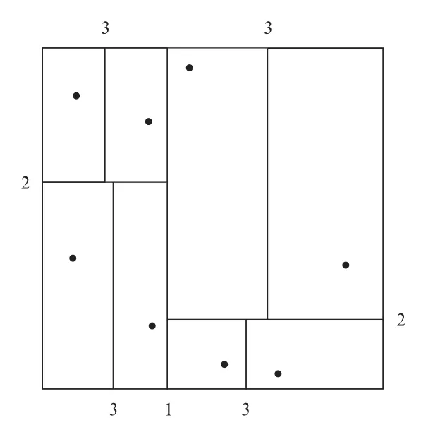 Figure 14.29 · PDF p. 702 · 2차원 공간을 level별 분할선으로 나누는 k-d tree space partitioning
Rectangular range query는 각 dimension의 interval을 지정한다. Search는 root에서 시작해 다음 규칙을 재귀적으로 적용한다.
- Internal node가 dimension
x의 split pointxi로 space를 나눈다면, query range가xi를 포함할 때 양쪽 child를 모두 search한다. - Query range가
xi왼쪽에만 있으면 left child만, 오른쪽에만 있으면 right child만 search한다. - Leaf에 도착하면 query range 안의 entries만 retrieve한다.
k-d-B tree는 k-d tree를 secondary storage에 맞게 확장해 internal node가 multiple children을 갖게 한 구조다. B-tree가 binary tree height를 줄이듯, k-d-B tree는 multidimensional partition tree의 height를 줄인다.
quadtrees는 2차원 space를 각 node에서 4개 quadrants로 나눈다. Points indexing에는 자연스럽지만, line segments, rectangles, polygons 같은 region object를 다루면 partition line을 가로지르는 object를 여러 subtrees에 중복 표현해야 할 수 있어 storage/query inefficiency가 생긴다.
R-tree는 points뿐 아니라 line segments, rectangles, polygons 같은 region objects를 index하기 위해 널리 쓰이는 balanced tree다. B+ tree처럼 indexed objects는 leaf nodes에 저장되지만, node마다 key range 대신 bounding box를 저장한다.
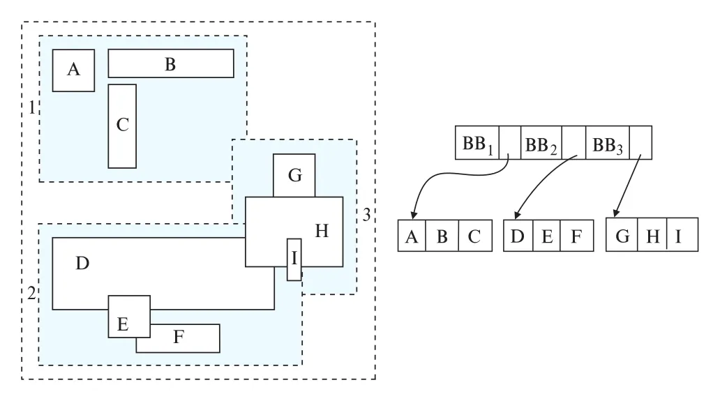 Figure 14.30 · PDF p. 704 · objects를 포함하는 bounding boxes와 그 boxes를 node entry로 저장하는 R-tree
R-tree의 bounding box는 axis-parallel rectangle이다. Leaf node의 bounding box는 그 leaf에 저장된 objects를 모두 포함하는 가장 작은 rectangle이고, internal node의 bounding box는 child nodes의 bounding boxes를 모두 포함하는 가장 작은 rectangle이다. Internal node는 child bounding box와 child pointer를 저장하고, leaf node는 indexed objects를 저장한다.
R-tree는 object를 한 번만 저장할 수 있고 node를 half full 이상으로 유지하기 쉬워 storage efficiency가 좋다. 단, bounding boxes가 overlap하면 query가 multiple paths를 search해야 하므로 어떤 alternative structures보다 query가 느릴 수 있다. 그래도 storage efficiency와 B-tree와의 유사성 때문에 spatial database에서 많이 쓰인다.
14.10.2 Indexing Temporal Data
temporal data는 tuple에 associated time period가 있는 data다. Tuple의 valid time interval은 그 fact가 유효한 기간을 나타낸다. 예를 들어 course ID의 title이 어느 시점에 바뀌면 같은 course ID에 대해 서로 다른 title tuples가 각자의 valid time interval을 가질 수 있다.
Time interval은 start time과 end time을 가지며, 각 endpoint가 open인지 closed인지도 표현해야 한다. 현재 유효한 tuple은 end time을 conceptual infinity로 둘 수 있고, 실제 구현에서는 9999-12-31 00:00 같은 매우 큰 time으로 표현할 수 있다.
어떤 fact의 valid period가 여러 disconnected intervals라면, 각 interval을 가진 여러 tuples로 표현할 수 있다. 따라서 indexing 논의에서는 single time interval을 가진 tuple만 고려해도 된다.
Attribute a = v이고 time point t1에서 유효한 tuple을 찾으려면 단순히 a index만으로는 부족할 수 있다. a = v인 모든 tuples를 가져온 뒤 time interval이 t1을 포함하는지 검사해야 하기 때문이다.
한 해결책은 tuple을 2차원 object로 보고 spatial index를 쓰는 것이다.
| dimension | 의미 |
|---|---|
| attribute dimension | indexed attribute a의 value v |
| time dimension | tuple의 valid time interval |
이 관점에서는 temporal tuple이 attribute value와 time interval로 이루어진 line segment가 되고, R-tree 같은 spatial index를 사용할 수 있다.
문제는 current tuple의 end time이 infinity라는 점이다. 매우 큰 bounding box는 spatial index 성능을 나쁘게 만들 수 있다. 원문은 다음 해결책을 제시한다.
| tuple 종류 | index strategy |
|---|---|
| current tuples, end time = infinity | 별도 B+ tree index on (a, start_time) |
| non-current tuples, finite interval | R-tree 같은 spatial index |
Time point lookup은 두 indices를 모두 search한다. Current-tuple index에서는 a = v and start_time <= ti range query를 수행하고, non-current tuple은 spatial index에서 interval containment을 찾는다.
Temporal interval에는 interval B+ tree 같은 specialized index도 사용할 수 있다. 다만 많은 DBMS는 새로운 interval index를 구현하기보다 이미 있는 R-tree를 사용하는 편이 단순하다. Temporal primary key constraint, 즉 같은 primary key value를 가진 tuples의 valid intervals가 overlap하면 안 되는 조건도 temporal index로 효율적으로 검사할 수 있다.
14.11 Summary
Chapter 14의 핵심 요약은 “index는 access path이며, workload에 맞게 구조를 골라야 한다”는 것이다.
dense index는 모든 search-key value에 entry를 두고,sparse index는 일부 values에만 entry를 둔다. Sparse index는 clustering index일 때만 가능하다.clustering index는 file의 sort order와 index search key order가 같고,secondary index는 다른 search key에 대한 dense index다. Secondary index는 read query를 빠르게 하지만 modifications에 overhead를 준다.B+ tree index는 balanced tree이며 모든 root-to-leaf path length가 같다. Disk block 크기에 맞춘 큰 fanout 덕분에 binary tree보다 훨씬 짧고, lookup/insert/delete가 logarithmic I/O로 동작한다.- B+ tree insertion은 leaf split과 parent insertion을, deletion은 coalesce/redistribution/root shrink를 처리해야 한다.
- B+ tree는 record pointers를 저장하는 index로도, actual records를 leaf level에 저장하는 file organization으로도 사용할 수 있다.
- B-tree는 key 중복을 줄이지만 fanout 감소와 deletion 복잡도 때문에 실제 DBMS에서는 B+ tree가 훨씬 널리 쓰인다.
hash index는 equality search에 강하지만 range query에는 약하다. Bucket overflow, skew, static hashing의 growth 문제를 고려해야 한다.- Multi-attribute query는 multiple single-key indices intersection, composite search key, covering index, bitmap index, R-tree 등 여러 선택지가 있다.
LSM tree와buffer tree는 high write/insert rate를 위해 B+ tree의 random write cost를 줄이려는 write-optimized index structures다.bitmap index는 low-cardinality attributes와 multiple predicates가 많은 analytic workload에서 bitmap intersection으로 강력하다.k-d tree,k-d-B tree,quadtree,R-tree는 spatial data를 위한 multidimensional index이며, temporal intervals도 spatial 관점으로 index할 수 있다.
Review Terms 관점에서 검색성을 위해 남겨 둘 핵심 용어는 다음과 같다.
| 묶음 | 핵심 용어 |
|---|---|
| index basics | ordered indices, hash indices, search key, access types, access time, insertion time, deletion time, space overhead |
| ordered index | clustering index, primary index, nonclustering index, secondary index, index-sequential file, dense index, sparse index, multilevel index |
| B+ tree | B+ tree index, balanced tree, leaf nodes, nonleaf nodes, internal nodes, range queries, node split, node coalesce, redistribution, uniquifier |
| extensions | prefix compression, bulk loading, bottom-up B+ tree construction, B-tree, covering index |
| hash/write optimized | hash function, bucket, overflow chaining, closed addressing, static hashing, dynamic hashing, LSM tree, stepped-merge index, buffer tree |
| bitmap/spatial/temporal | bitmap index, bitmap intersection, k-d tree, k-d-B tree, quadtree, R-tree, bounding box, temporal index, time interval, open interval, closed interval |
Practice Exercises와 Exercises는 dense/sparse 선택, clustering/secondary 차이, B+ tree insert/delete 시뮬레이션, prefix compression, secondary index relocation 문제, write-optimized index trade-off, bitmap construction, spatial/temporal index 선택을 묻는다. 이 장을 이해했다면 “어떤 query/workload에 어떤 index를 만들 것인가”를 비용과 update overhead까지 포함해 설명할 수 있어야 한다.
연결 관계
- Chapter 13 Data Storage Structures: file organization, block/page layout, database buffer, B+ tree file organization, large object storage와 직접 연결된다.
- Chapter 15 Query Processing: index는 selection, join, sort/range scan의 physical access path로 사용되며, query plan cost의 핵심 입력이 된다.
- Chapter 16 Query Optimization: optimizer는 available indices, selectivity, clustering 여부, covering 여부, bitmap intersection 가능성을 보고 evaluation plan을 선택한다.
- Chapter 19 Recovery System: B+ tree page split/merge, LSM merge, index updates도 transaction/recovery protocol 안에서 atomic/durable하게 처리되어야 한다.
- Chapter 24 Advanced Indexing Techniques: Bloom filter, LSM variants, bitmap implementation, spatial index, dynamic hashing을 더 깊게 다룬다.
오해하기 쉬운 내용
search key는 primary key가 아니다. Search key는 index lookup에 쓰는 attribute set이며, 중복될 수 있다.primary index라는 말은 primary key index라는 뜻이 아니라 clustering index를 뜻할 수 있다. 이 책에서는 clustering index와 primary index가 같은 의미로 쓰인다.- Sparse index는 아무 index에나 쓸 수 없다. File이 search key order로 정렬된 clustering index에서만 중간 records를 sequential scan으로 찾을 수 있다.
- B+ tree의 nonleaf key는 record 자체가 아니다. Separator 역할을 하므로 deletion 뒤 leaf에 없는 key가 nonleaf에 남을 수 있다.
- B-tree와 B+ tree는 이 책에서는 다른 구조다. 하지만 실무 문서에서는 B-tree라고 부르면서 실제로 B+ tree를 의미하는 경우가 많다.
- Hash index는 equality search에는 좋지만 range query에는 부적합하다. Hash function은 key order를 보존하지 않는다.
- Composite
(A, B)index는A = value또는A = value and B range에는 강하지만,A range and B range같은 일반 multidimensional range query에는 한계가 있다. - Bitmap index는 low-cardinality 단일 조건만 빠르게 하려고 쓰는 것이 아니라, 여러 conditions의 bitmap intersection을 빠르게 하기 위해 유용하다.
- LSM tree는 “tree 하나”가 아니라 memory/disk의 여러 sorted trees와 merge policy의 조합이다.
- R-tree bounding box는 object 자체가 아니라 object 또는 child boxes를 포함하는 최소 axis-parallel rectangle이다.
면접 질문
search key와 primary key/candidate key/superkey의 차이를 설명하라.- Dense index와 sparse index의 차이, 그리고 sparse index가 clustering index에서만 가능한 이유를 설명하라.
- Clustering index와 secondary index가 range scan과 update cost에 어떤 차이를 만드는가?
- Multilevel index가 binary search on index file보다 disk I/O를 줄이는 이유를 설명하라.
- B+ tree에서 leaf node와 nonleaf node의 역할,
fanout, leaf chain의 의미를 설명하라. - B+ tree equality lookup과 range query가 각각 어떻게 진행되는가?
- B+ tree insertion에서 leaf split과 nonleaf split의 separator key 처리 차이를 설명하라.
- B+ tree deletion에서
coalesce,redistribution, root shrink가 언제 일어나는가? - Nonunique search key를
uniquifier attribute로 unique composite key로 만드는 이유를 deletion cost 관점에서 설명하라. - B+ tree file organization에서 record relocation이 secondary index update를 비싸게 만드는 이유와 logical record identifier 해결책을 설명하라.
bulk loading과 bottom-up B+ tree construction이 tuple-at-a-time insertion보다 빠른 이유는 무엇인가?- B-tree와 B+ tree의 구조적 차이와 실제 DBMS가 B+ tree를 선호하는 이유를 설명하라.
- Hash index가 equality query에는 좋지만 range query에는 약한 이유를 설명하라.
- Composite index
(dept_name, salary)가 잘 처리하는 query와 잘 처리하지 못하는 query를 예로 들어 설명하라. - Covering index가 actual record fetch를 줄이는 방식과 composite key index와의 차이를 설명하라.
- LSM tree에서 insert, lookup, delete entry, merge가 어떻게 동작하는지 설명하라.
- Buffer tree가 insert cost를 amortize하는 방식과 LSM tree 대비 trade-off를 설명하라.
- Bitmap index에서
gender=f AND income_level=L2같은 query가 bitwise AND로 처리되는 과정을 설명하라. - k-d tree와 R-tree가 각각 어떤 spatial data/query에 적합한지 설명하라.
- Temporal data의 current tuples를 별도 B+ tree index에 두고 non-current tuples를 R-tree에 두는 이유를 설명하라.