개요
query processing은 고수준 질의 언어로 작성된 query를 실제 file system/storage level에서 실행 가능한 작업들의 흐름으로 바꾸고, 그중 비용이 낮은 실행 방식을 골라 결과를 계산하는 전체 활동이다. 사용자는 SQL처럼 사람이 읽기 쉬운 언어로 질의를 쓰지만, DBMS 내부는 이를 extended relational algebra, evaluation primitive, query-evaluation plan, physical operator, access path로 바꾸어 실행한다.
Chapter 15의 초점은 “개별 relational-algebra operation을 어떻게 실행하고, 그 비용을 어떻게 추정하는가”다. Chapter 16의 query optimization은 여기서 배운 selection, sorting, join, aggregation, pipelining 등의 실행 알고리즘과 cost model을 재료로 여러 plan 중 하나를 선택한다.
핵심 개념
query processing은 parsing/translation, optimization, evaluation으로 이어지는 실행 준비와 실행 전체를 뜻한다.parser and translator는 SQL query의 syntax와 relation/view 이름을 확인하고, 내부 표현인 relational-algebra expression 또는 annotated parse tree로 바꾼다.query optimization은 같은 의미의 여러 relational expression과 여러 physical algorithm 중 estimated cost가 낮은query-evaluation plan을 고르는 단계다.evaluation primitive는 relational-algebra operation에 “어떤 algorithm/access path/index를 사용할지”가 주석처럼 붙은 실행 단위다.query-evaluation plan또는query-execution plan은 evaluation primitives의 sequence/tree이며, query-execution engine이 실제로 실행한다.- Query cost는 response time 자체보다 보통 total resource consumption으로 근사한다. 이 장의 기본 모델은
block transfer수와random I/O access수를 중심으로 한다. - Cost formula의 기본형은
b * tT + S * tS다. 여기서b는 transferred blocks,S는 random I/O accesses,tT는 block transfer time,tS는 block access latency다. - Memory buffer size
M, buffer residence, SSD/main-memory latency, CPU tuple/index/operator cost는 실제 optimizer에서 중요하지만, 이 장의 기본 설명에서는 단순화를 위해 일부를 생략하거나 parameter로 둔다.
세부 정리
15.1 Overview
Query processing은 크게 세 단계로 나뉜다.
| 단계 | 역할 | 산출물 |
|---|---|---|
| parsing and translation | SQL query를 검사하고 내부 표현으로 변환 | parse tree, relational-algebra expression |
| optimization | 같은 의미의 여러 표현/알고리즘 중 비용이 낮은 plan 선택 | query-evaluation plan |
| evaluation | 선택된 plan을 query-execution engine이 실행 | query output |
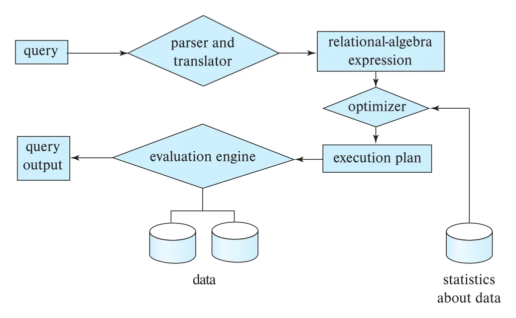 Figure 15.1 · PDF p. 719 · query가 parser/translator, optimizer, evaluation engine을 거쳐 output이 되는 흐름
SQL은 사람에게 적합하지만 DBMS 내부 표현으로는 불편하다. 그래서 parser는 query syntax를 확인하고, query에 등장하는 relation name이 실제 database에 존재하는지 검증하며, query를 parse tree로 만든 뒤 relational-algebra expression으로 변환한다. Query가 view를 사용하면 일반 view는 그 view definition의 relational-algebra expression으로 치환된다. 반면 materialized view는 이미 계산되어 저장된 relation이므로, 정의식을 다시 펼치는 대신 저장된 결과를 사용할 수 있다.
같은 SQL query도 여러 relational-algebra expression으로 번역될 수 있다. 예를 들어 다음 query는 salary만 projection한 뒤 selection할 수도 있고, selection을 먼저 수행한 뒤 projection할 수도 있다.
select salary
from instructor
where salary < 75000;두 expression은 같은 결과를 낼 수 있지만 실행 비용은 다를 수 있다. Selection을 구현할 때도 relation 전체를 scan할지, salary 위의 B+ tree index를 사용할지, clustering 여부를 고려할지에 따라 비용이 달라진다.
Relational-algebra expression만으로는 “무엇을 계산하는가”만 일부 지정할 뿐, “어떻게 계산하는가”를 충분히 지정하지 않는다. 따라서 DBMS는 operation마다 사용할 algorithm, index, access path를 명시한 evaluation primitive를 만들고, 이 primitive들의 조합을 query-evaluation plan으로 실행한다.
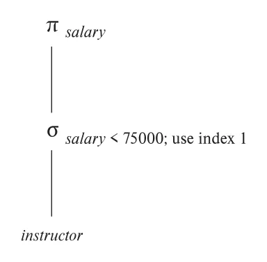 Figure 15.2 · PDF p. 720 · salary selection에 특정 index를 쓰도록 주석이 붙은 query-evaluation plan
사용자는 효율적인 plan을 암시하도록 SQL을 작성할 책임이 없다. DBMS가 여러 equivalent expression과 physical algorithm을 비교해 plan을 선택해야 하며, 이것이 query optimization이다. Chapter 15는 plan 후보를 구성하는 개별 operation의 실행 방법과 cost estimation을 다루고, Chapter 16은 이 정보를 사용해 plan을 선택하는 optimizer를 다룬다.
15.2 Measures of Query Cost
같은 query에도 여러 evaluation plan이 가능하므로, DBMS는 각 operation cost를 추정하고 이를 합쳐 plan cost를 비교해야 한다. Query evaluation cost에는 여러 resource가 들어간다.
| resource | 의미 |
|---|---|
| disk access / storage access | block read/write, random I/O, sequential transfer |
| CPU time | tuple 검사, index entry 처리, expression/operator/function 계산 |
| communication cost | parallel/distributed DB에서 node 간 data movement 비용 |
| memory buffer | operator가 사용할 수 있는 buffer 크기 M, cache/buffer residence |
초기 cost model은 magnetic disk에서 I/O cost가 지배적이라는 가정에 기반했다. SSD와 large main memory가 보편화되면서 CPU cost와 memory hierarchy도 중요해졌지만, 이 장은 설명을 단순하게 하기 위해 주로 block transfer와 random I/O access를 사용한다. 실제 PostgreSQL 같은 DBMS는 tuple당 CPU cost, index entry 처리 cost, operator/function 실행 cost를 별도 parameter로 두고 cost를 계산한다.
이 장의 기본 I/O cost model은 다음과 같다.
| 기호 | 의미 |
|---|---|
b | storage에서 transfer되는 block 수 |
S | random I/O access 수 |
tT | 한 block을 transfer하는 시간 |
tS | random block access latency. magnetic disk에서는 seek + rotational latency, SSD에서는 I/O request 후 첫 byte가 올 때까지의 latency |
Magnetic disk에서는 tS가 tT보다 훨씬 커서 random I/O를 줄이는 것이 매우 중요하다. SSD는 물리적 seek는 없지만 request latency가 있고, sequential throughput과 random read 처리량의 차이가 여전히 존재한다. Main memory에서는 disk block이 아니라 cache line 단위 접근이 핵심이 되며, memory latency와 CPU cache miss가 중요해진다.
Block read와 block write도 비용이 다를 수 있다. Magnetic disk에서는 write 후 verify를 위해 다시 읽는 과정 때문에 write가 read보다 비쌀 수 있고, flash storage에서는 erase/write 특성이 영향을 준다. 이 장의 단순 모델에서는 이런 차이를 대체로 무시하거나 필요한 곳에서만 별도 반영한다. 또한 operation의 final result를 disk에 쓰는 비용은 기본 operation cost에 항상 포함하지 않고, 필요한 경우 별도로 계산한다.
Cost estimation에서 M은 operator가 사용할 수 있는 main-memory buffer block 수다. Data가 buffer 안에 다 들어가면 disk를 다시 읽을 필요가 없고, 반대로 buffer가 거의 없으면 같은 data를 여러 번 읽을 수 있다. 실제 DBMS는 query 전체에 사용할 memory를 여러 concurrent operators 사이에 나누어야 한다.
Buffer residence도 중요한 문제다. 어떤 block이 이미 in-memory buffer에 있으면 실제 disk access cost는 추정보다 낮다. 하지만 optimizer가 plan 선택 시점에 buffer 내용을 정확히 알기는 어렵다. 그래서 DBMS는 heuristic을 쓴다. 예를 들어 PostgreSQL은 random page read cost를 실제보다 낮게 잡아 상당수 page가 cache에 있을 가능성을 반영하고, 대부분의 DBMS는 B+ tree internal nodes가 자주 접근되므로 buffer에 있다고 가정한다. 이 경우 B+ tree traversal은 root-to-leaf 전체 random I/O가 아니라 leaf node 접근 1회 정도로 단순화할 수 있다.
response time은 사용자가 실제로 기다리는 wall-clock time이므로 가장 직관적인 cost처럼 보이지만, optimizer가 정확히 예측하기 어렵다.
| response time 예측이 어려운 이유 | 설명 |
|---|---|
| buffer 시작 상태 의존 | query 시작 시 어떤 blocks가 cache/buffer에 있는지 알기 어렵다. |
| data layout/parallelism 의존 | 여러 disk/SSD/channel에 access가 어떻게 분산되는지에 따라 wall-clock time이 달라진다. |
| resource consumption과 충돌 | 더 많은 disk reads를 병렬로 수행하면 response time은 줄어도 전체 resource 사용량은 늘 수 있다. |
따라서 optimizer는 일반적으로 response time 자체를 직접 최소화하기보다, plan의 total resource consumption을 최소화하려 한다. 이 장의 disk access time model은 그런 resource-consumption 기반 query cost model의 대표 예다.
15.3 Selection Operation
selection operation은 file scan이라는 가장 낮은 수준의 access operator 위에서 구현된다. File scan은 selection condition을 만족하는 records를 locate/retrieve하는 search algorithm이다. Relation이 하나의 dedicated file에 저장되어 있으면 file scan은 relation 전체 또는 필요한 부분을 읽으며 조건을 검사한다.
15.3.1 Selections Using File Scans and Indices
가장 기본 selection algorithm은 A1 (linear search)다. Linear search는 file의 모든 block을 scan하고, 각 record가 selection condition을 만족하는지 검사한다. 첫 block을 읽기 위해 initial seek가 필요하고, file blocks가 contiguous하지 않으면 추가 seek가 필요할 수 있지만, 기본 cost model은 단순화를 위해 이를 무시한다.
Linear search는 ordering, index availability, selection condition 형태와 무관하게 항상 적용 가능하다. 다른 selection algorithm은 특정 ordering이나 index가 있을 때 훨씬 빠를 수 있지만, 적용 범위가 제한된다. 그래서 query processing에서 linear scan은 가장 단순하고 보편적인 fallback access path다.
Index는 data를 찾는 경로를 제공하므로 access path라고 불린다. Chapter 14의 clustering index는 file physical order와 index search-key order가 대응되어 range scan에 유리하고, secondary index 또는 nonclustering index는 file physical order와 독립적이어서 matching records가 여러 blocks에 흩어질 수 있다.
Index를 사용하는 search algorithm은 index scan이라고 부른다. Selection predicate는 어떤 index를 사용할지 결정하는 기준이 된다. Figure 15.3은 대표 selection algorithms의 cost estimate를 비교한다. 여기서 br은 relation file block 수, hi는 B+ tree height, n은 fetched records 수, b는 matching records가 들어 있는 block 수다.
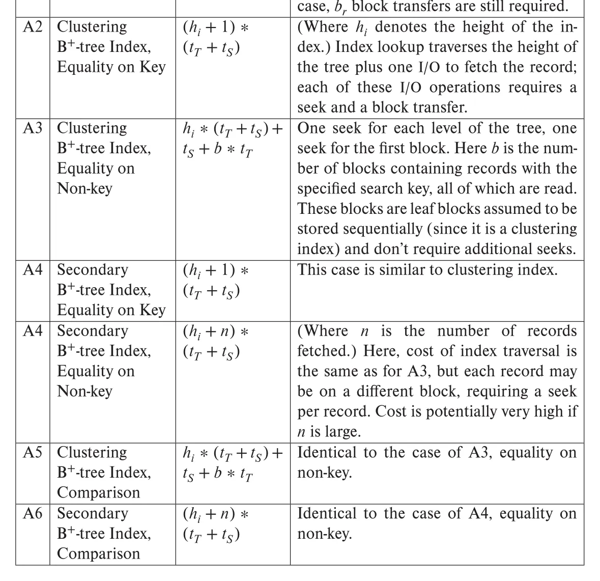 Figure 15.3 · PDF p. 725 · linear search와 B+ tree 기반 selection algorithms의 cost estimates
Selection algorithms A1-A6의 의미는 다음과 같다.
| algorithm | 조건/구조 | 핵심 동작 | 주의점 |
|---|---|---|---|
A1 linear search | 모든 file, 모든 selection | 모든 block/record 검사 | 항상 가능하지만 relation 전체 scan |
A1 equality on key | key equality | key는 최대 1개 record만 match하므로 찾으면 중단 가능 | 평균적으로 file 절반 scan, worst case는 전체 scan |
A2 clustering B+ tree index, equality on key | clustering index + key equality | index lookup 후 single record fetch | B+ tree file organization이면 leaf에 record가 있어 한 access를 줄일 수 있음 |
A3 clustering B+ tree index, equality on non-key | clustering index + duplicate 가능 | 같은 key의 records가 file에 consecutive하게 저장되어 sequential read | matching block 수 b가 비용을 좌우 |
A4 secondary B+ tree index, equality | secondary index + equality | key equality는 single record, non-key equality는 여러 record pointer fetch | non-key이면 each record may be on a different block라 매우 비쌀 수 있음 |
A5 clustering B+ tree index, comparison | clustering ordered index + <, <=, >, >= | boundary를 찾고 file scan | < v, <= v는 beginning부터 scan하므로 index lookup이 유용하지 않을 수 있음 |
A6 secondary B+ tree index, comparison | secondary ordered index + comparison | lowest-level index blocks를 scan하고 record pointers로 fetch | 많은 tuple이 선택되면 linear search보다 비쌀 수 있음 |
secondary index가 non-key equality나 comparison에 쓰일 때 가장 큰 위험은 random I/O 폭발이다. Index entries는 순서대로 읽을 수 있어도 실제 records는 disk file 여기저기에 흩어져 있을 수 있다. 따라서 selected tuple 수가 크면 (hi + n) * (tT + tS)처럼 record마다 random access가 들어가 linear scan보다 느릴 수 있다. Optimizer가 selectivity를 잘못 추정하면 secondary index scan 선택이 오히려 나쁜 plan이 된다.
PostgreSQL의 bitmap index scan은 이 문제를 완화하는 hybrid algorithm이다. 이름은 bitmap index와 비슷하지만, Chapter 14의 bitmap index 자체를 scan한다는 뜻이 아니다. Secondary index로 matching index entries를 찾되 record를 즉시 fetch하지 않고, relation block 수만큼 bit를 둔 bitmap에 “matching tuple이 들어 있는 block”만 표시한다. 그 뒤 relation을 block order로 scan하면서 bit가 1인 block만 읽고, block 안에서 matching records를 찾는다.
secondary index entries -> block bitmap -> block-order relation scan이 방식은 worst case에서 linear scan보다 크게 나쁘지 않고, best case에서는 직접 secondary index pointer를 따라 random I/O를 반복하는 것보다 훨씬 싸다. 변형으로는 matching index entries를 모아 record pointer 순서로 sort한 뒤 block order로 fetch하는 방식도 가능하지만, bitmap이 sorting보다 더 쌀 수 있다.
15.3.2 Selections Involving Comparisons
Comparison selection sigma_A<=v(r) 같은 질의는 index 종류와 비교 방향에 따라 달라진다. Clustering ordered index에서 A >= v 또는 A > v는 index로 시작 위치를 찾고 그 지점부터 file 끝까지 scan하면 된다. 반면 A < v 또는 A <= v는 file beginning부터 조건을 만족하는 마지막 지점까지 scan하면 되므로, 굳이 index lookup을 하지 않아도 된다.
Secondary ordered index는 <, <=, >, >= 모두에서 lowest-level index block을 범위 방향으로 scan할 수 있다. 하지만 실제 record fetch는 pointer를 따라가야 하므로 selected records가 많으면 random I/O가 커진다. 그래서 secondary index comparison은 “매우 작은 fraction만 선택될 때” 유리하고, 많은 tuple이 선택되면 linear scan이 낫다.
15.3.3 Implementation of Complex Selections
복합 selection predicate는 conjunction, disjunction, negation으로 구성된다.
| 형태 | relational algebra | 의미 |
|---|---|---|
| conjunction | sigma_theta1 AND theta2 AND ... AND thetan(r) | 모든 simple condition을 만족 |
| disjunction | sigma_theta1 OR theta2 OR ... OR thetan(r) | simple condition 중 하나 이상 만족 |
| negation | sigma_NOT theta(r) | 조건 theta가 false인 tuples |
Conjunctive selection은 여러 방식으로 구현할 수 있다.
| algorithm | 핵심 아이디어 | 적합한 경우 |
|---|---|---|
A7 conjunctive selection using one index | 가장 selective하거나 cost가 낮은 simple condition 하나에 A2-A6을 적용하고, 나머지 조건은 memory에서 검사 | 좋은 단일 access path가 하나 있을 때 |
A8 conjunctive selection using composite index | 여러 equality condition을 composite index로 직접 search | (A, B, ...) composite search key가 predicate와 잘 맞을 때 |
A9 conjunctive selection by intersection of identifiers | 각 조건의 index scan 결과 record pointers를 intersection하고 실제 records fetch | 여러 condition에 각각 index가 있고 pointer intersection이 작을 때 |
A9에서 pointer list를 sort하면 같은 block에 대한 pointers가 모이고, blocks를 sorted order로 읽을 수 있어 disk-arm movement와 random I/O를 줄일 수 있다. 이 지점에서 Section 15.4의 sorting algorithm이 selection processing과 연결된다.
Disjunctive selection은 A10 disjunctive selection by union of identifiers로 처리할 수 있다. 각 OR 조건에 access path가 있으면 index scan 결과 pointers를 union한 뒤 records를 fetch한다. 하지만 OR 조건 중 하나라도 access path가 없으면, 어차피 relation을 scan해야 하므로 전체 linear scan 중 disjunctive condition을 검사하는 편이 일반적으로 낫다.
15.4 Sorting
Sorting은 DBMS에서 두 가지 이유로 중요하다. 첫째, SQL query가 ORDER BY처럼 sorted output을 요구할 수 있다. 둘째, join, duplicate elimination, grouping/aggregation 같은 relational operations는 input이 sorted되어 있으면 효율적으로 구현될 수 있다.
Index를 sort key 위에 만들고 그 index 순서대로 relation을 읽으면 logical sorted order를 얻을 수 있다. 그러나 secondary index를 따라 sorted order로 tuple을 읽으면 record마다 disk seek가 발생할 수 있다. 즉 index는 logical order를 주지만 physical order를 보장하지 않는다. 그래서 relation이 memory보다 클 때는 records를 물리적으로 정렬하는 external sorting이 필요하다.
15.4.1 External Sort-Merge Algorithm
external sorting은 relation이 main memory에 모두 들어가지 않을 때의 sorting이다. 가장 일반적인 방법은 external sort-merge algorithm이다. M은 sorting에 사용할 수 있는 main-memory buffer blocks 수다.
External sort-merge는 두 단계로 진행된다.
| 단계 | 동작 | 결과 |
|---|---|---|
| run generation | relation에서 최대 M blocks씩 읽고, memory에서 sort한 뒤 sorted run Ri로 write | 여러 sorted runs |
| merge stage | 각 run의 input buffer에서 가장 작은 tuple을 골라 output buffer에 쓰고, 빈 input buffer는 다음 block으로 채움 | 전체 sorted relation |
Merge stage에서 runs 수 N이 M보다 작으면 각 run에 input buffer 1개와 output buffer 1개를 둘 수 있어 한 번의 N-way merge로 끝난다. 하지만 relation이 훨씬 크면 initial runs 수가 M 이상이므로, 한 번에 M - 1개의 runs만 merge하고 여러 merge passes를 반복한다. 각 pass는 runs 수를 대략 M - 1배 줄이고, runs 수가 M보다 작아지면 final pass가 sorted output을 만든다.
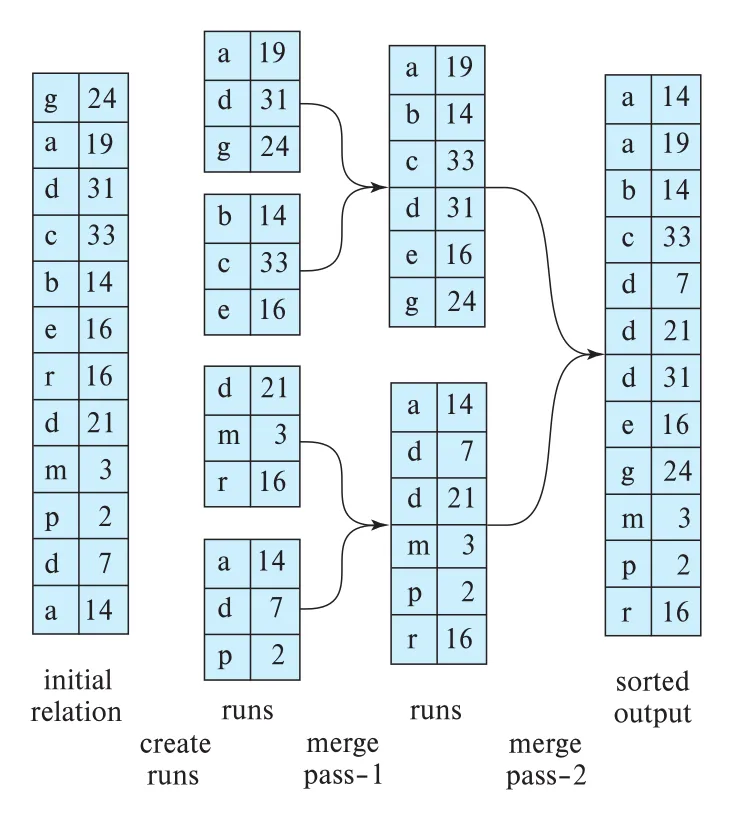 Figure 15.4 · PDF p. 732 · initial relation에서 sorted runs를 만들고 여러 merge pass로 sorted output을 생성하는 external sort-merge
15.4.2 Cost Analysis of External Sort-Merge
br을 relation r의 block 수라고 하자. Run generation은 모든 block을 한 번 읽고 sorted run으로 한 번 쓰므로 2br block transfers가 든다. Initial runs 수는 ceil(br / M)이다.
Merge pass에서 seek 수를 줄이기 위해 각 input run과 output에 한 block씩이 아니라 bb buffer blocks씩 할당할 수 있다. 그러면 한 pass에서 merge할 수 있는 run 수는 floor(M / bb) - 1이다. 필요한 merge pass 수는 다음과 같다.
Final pass의 output은 바로 query pipeline으로 넘기거나 최종 결과로 사용할 수 있으므로, final sorted result를 disk에 다시 쓰는 비용은 보통 제외한다. 이때 external sort의 block transfer 수는 원문 단순화 기준으로 다음과 같다.
Seek cost도 별도로 고려한다. Run generation은 각 run을 읽고 쓰기 위한 seeks가 필요하고, 각 merge pass는 input runs를 읽기 위한 seeks와 output write seeks가 필요하다. 원문이 Figure 15.4 예시에 적용한 seek 수 식은 다음과 같다.
정리하면 external sort-merge의 cost를 좌우하는 것은 relation size br, available memory M, per-run buffer size bb다. M이 클수록 initial runs가 줄고 merge fan-in이 커져 passes가 줄어든다. bb를 크게 잡으면 sequential I/O 묶음이 커져 seek가 줄지만, 동시에 merge할 수 있는 runs 수가 줄어 pass 수가 늘 수 있다.
15.5 Join Operation
Join은 query processing에서 가장 비용이 큰 operation 중 하나다. 이 절은 nested-loop join, block nested-loop join, indexed nested-loop join, merge join, hash join, hybrid hash join을 비교한다. 원문은 student ⋈ takes를 running example으로 사용하며, student는 5000 records/100 blocks, takes는 10,000 records/400 blocks라고 가정한다.
equi-join은 r ⋈ r.A = s.B s처럼 양쪽 relation의 attribute 값이 같은 tuple 쌍을 찾는 join이다. natural join은 common attributes를 기준으로 equi-join한 뒤 duplicate attributes를 제거하는 특수한 경우로 볼 수 있다.
15.5.1 Nested-Loop Join
nested-loop join은 가장 일반적인 join algorithm이다. Outer relation r의 각 tuple마다 inner relation s의 모든 tuple을 검사하고, join condition theta를 만족하면 결과에 tr · ts를 추가한다.
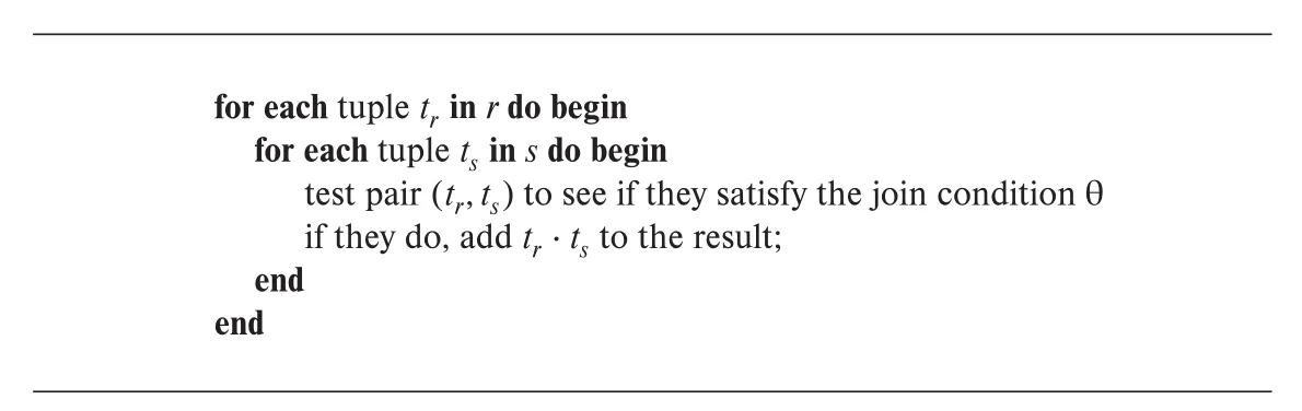 Figure 15.5 · PDF p. 734 · outer tuple마다 inner relation 전체를 검사하는 nested-loop join
Nested-loop join은 index가 없어도 되고, join condition이 equi-join이 아니어도 된다. Selection의 linear scan처럼 범용성이 장점이다. 단점은 모든 tuple pair를 검사하므로 매우 비싸다는 점이다.
| 상황 | block transfers | seeks | 의미 |
|---|---|---|---|
| worst case, buffer가 relation당 1 block 수준 | nr * bs + br | nr + br | outer tuple마다 inner relation scan |
| both relations fit in memory | br + bs | 2 | 각 relation을 한 번씩만 읽음 |
| inner relation만 memory에 fit | br + bs | 2 | inner를 한 번 읽어 memory에 둔 뒤 outer scan |
Nested-loop join에서는 어느 relation을 outer로 둘지가 중요하다. Inner가 매번 scan되므로, 작은 relation이 inner에 들어가 memory에 fit하면 큰 이득이 있다. 반대로 memory가 작고 index도 없으면 tuple 수가 작은 relation을 outer로 선택하는 것이 block transfer를 줄일 수 있다.
15.5.2 Block Nested-Loop Join
block nested-loop join은 tuple 단위가 아니라 block 단위로 중첩 loop를 수행한다. Outer relation의 한 block Br와 inner relation의 한 block Bs를 memory에 두고, 두 block 안의 모든 tuple pair를 검사한다.
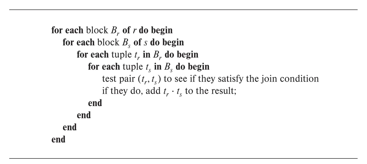 Figure 15.6 · PDF p. 735 · outer block과 inner block의 모든 tuple pair를 검사하는 block nested-loop join
Block nested-loop join은 basic nested-loop join보다 훨씬 낫다. Inner relation을 outer tuple마다 읽는 대신 outer block마다 읽기 때문이다.
| 기준 | worst-case cost |
|---|---|
| block transfers | br * bs + br |
| seeks | 2 * br |
Memory가 M blocks 있으면 outer relation을 한 block씩이 아니라 M - 2 blocks씩 읽을 수 있다. Inner block buffer와 output buffer를 하나씩 남겨 두기 때문이다. 이 경우 inner relation scan 횟수는 br이 아니라 ceil(br / (M - 2))가 된다.
추가 최적화도 있다. Natural/equi-join에서 inner join attribute가 key이면 첫 match를 찾은 뒤 inner scan을 멈출 수 있다. Inner loop를 forward/backward로 번갈아 scan하면 이전 scan에서 buffer에 남은 block을 재사용할 가능성이 커진다. Inner relation의 join attribute에 index가 있으면 다음 indexed nested-loop join으로 넘어갈 수 있다.
15.5.3 Indexed Nested-Loop Join
indexed nested-loop join은 inner relation의 join attribute에 index가 있을 때 inner file scan을 index lookup으로 바꾼다. Outer relation의 각 tuple tr에 대해, join condition을 만족하는 inner tuples를 찾는 것은 결국 inner relation에 대한 selection과 같다. 예를 들어 student ⋈ takes에서 student tuple의 ID = 00128이면, inner takes에서 ID = 00128인 tuples를 index로 찾는다.
Cost는 outer relation을 읽는 비용과 outer tuple마다 inner index lookup을 수행하는 비용의 합으로 본다.
| 기호 | 의미 |
|---|---|
br | outer relation r의 block 수 |
nr | outer relation r의 tuple 수 |
c | inner relation s에서 join condition으로 selection 1회를 수행하는 비용 |
양쪽 relation 모두 index가 있다면 tuple 수가 적은 relation을 outer로 두는 것이 보통 유리하다. 하지만 indexed nested-loop join이 항상 좋은 것은 아니다. Outer tuple 수가 많고 inner index가 secondary index라서 record fetch가 random I/O를 많이 유발하면, block nested-loop join이나 hash join보다 느려질 수 있다. 반대로 outer input이 selection으로 매우 작아진 상태라면 indexed nested-loop join이 매우 빠르다.
15.5.4 Merge Join
merge join 또는 sort-merge join은 natural join과 equi-join에 사용할 수 있다. 두 input relation이 join attributes 위에서 sorted되어 있으면, merge sort의 merge 단계처럼 양쪽 pointer를 앞으로 움직이며 같은 join value를 가진 tuple groups를 결합한다.
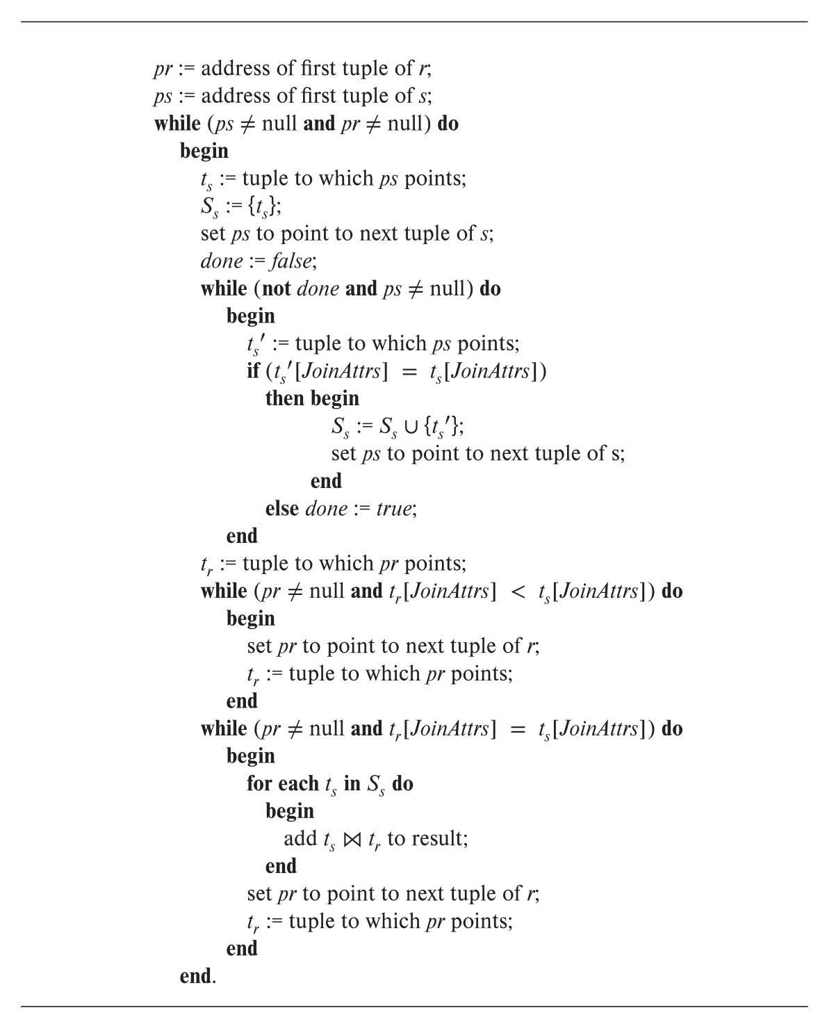 Figure 15.7 · PDF p. 738 · sorted relations를 join attribute 순서로 훑는 merge join algorithm
Merge join은 각 relation에 pointer를 하나씩 두고, join attribute 값이 작은 쪽 pointer를 앞으로 이동시킨다. 어떤 join value에 대해 한 relation의 matching group Ss를 memory에 읽고, 다른 relation의 같은 join value tuples와 결합한다. 원문 알고리즘은 각 Ss가 memory에 fit한다고 가정한다. 특정 join value의 group이 너무 크면 해당 group에는 block nested-loop join 같은 다른 기법을 적용할 수 있다.
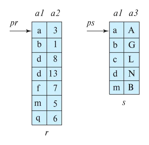 Figure 15.8 · PDF p. 739 · join attribute a1 기준으로 정렬된 두 relation과 merge join pointer 진행
이미 sorted되어 있다면 merge join은 각 block을 한 번씩만 읽는다.
| 조건 | block transfers | seeks |
|---|---|---|
| inputs already sorted, groups fit in memory | br + bs | ceil(br / bb) + ceil(bs / bb) |
| inputs not sorted | sort cost + br + bs | sort seek cost + merge seek cost |
정렬되지 않은 input에 merge join을 쓰려면 먼저 external sort-merge cost를 더해야 한다. Memory가 작으면 sort passes와 seeks가 폭증하고, memory가 충분하면 one merge step으로 끝나 비용이 크게 줄어든다. 이 절의 예시는 memory가 3 blocks일 때와 25 blocks일 때 sort+merge join cost가 크게 달라짐을 보여준다.
hybrid merge join은 한 relation은 sorted되어 있고, 다른 relation은 unsorted지만 join attribute에 secondary B+ tree index가 있을 때 사용할 수 있다. Sorted relation과 secondary index leaf entries를 merge해 먼저 sorted relation tuple과 unsorted relation tuple address를 결합한 중간 결과를 만든다. 그 중간 결과를 tuple address 순서로 다시 sort하면 unsorted relation records를 physical order로 효율적으로 fetch할 수 있다. 핵심은 secondary index를 따라 tuple을 하나씩 random fetch하는 비용을 줄이는 것이다.
15.5.5 Hash Join
hash join은 natural join과 equi-join에 사용하는 대표적 algorithm이다. Join attribute 값에 hash function h를 적용해 양쪽 relation을 같은 hash value partition으로 나눈다. Join condition을 만족하는 tuple pair는 반드시 같은 hash value를 가지므로, ri의 tuples는 si의 tuples와만 비교하면 된다.
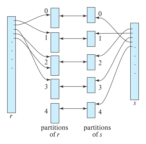 Figure 15.9 · PDF p. 742 · join attributes의 hash value로 relation r과 s를 같은 번호 partitions로 나누는 hash partitioning
15.5.5.1 Basics
Hash join은 보통 두 phase로 이해한다.
| phase | 동작 |
|---|---|
| partitioning | r과 s를 join attributes의 hash value로 r0...rnh, s0...snh에 분할 |
| build/probe | build input partition si를 memory에 읽어 hash index를 만들고, probe input partition ri의 tuples로 lookup |
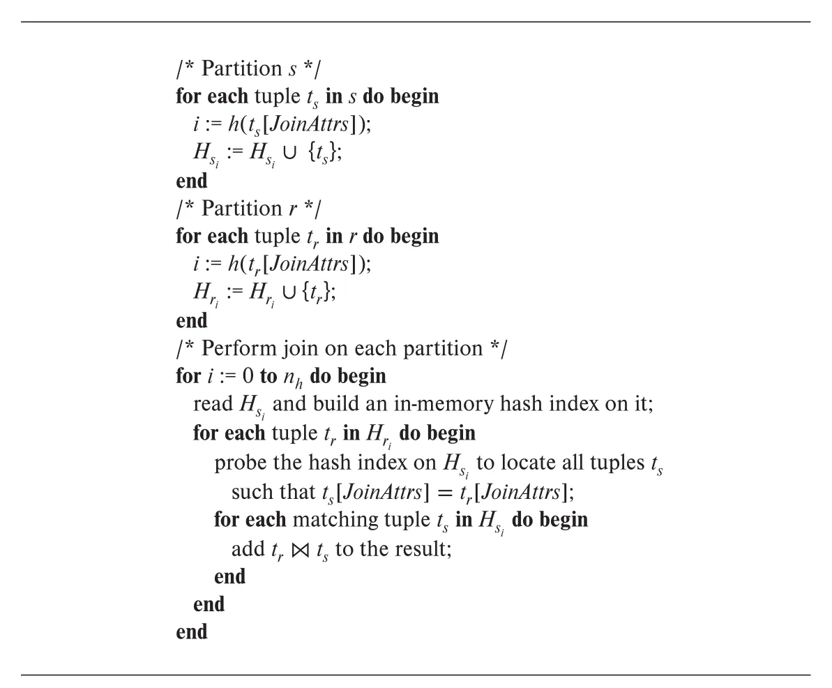 Figure 15.10 · PDF p. 743 · partitioning 후 build partition에 in-memory hash index를 만들고 probe하는 hash join
s는 build input, r은 probe input이라고 부른다. Build partition과 그 hash index가 memory에 들어가야 하므로, 더 작은 relation을 build input으로 두는 것이 좋다. Partitioning에 쓰는 hash function h와, memory 안의 hash index를 만들 때 쓰는 hash function은 달라야 한다. 두 함수 모두 join attributes에 적용되지만 목적이 다르다.
nh는 build relation의 각 partition si와 그 hash index가 memory에 들어갈 만큼 커야 한다. 단, probe relation partitions는 memory에 fit할 필요가 없다. Build input size가 bs blocks이면 단순하게 nh >= ceil(bs / M) 정도가 필요하고, 실제로는 hash index overhead까지 고려해 더 크게 잡는다.
15.5.5.2 Recursive Partitioning
recursive partitioning은 한 번의 partitioning으로 build partitions가 memory에 들어가지 않을 때 반복적으로 partition을 더 쪼개는 방식이다. 한 pass에서 만들 수 있는 partitions 수는 output buffer blocks 수로 제한된다. 각 pass는 이전 bucket을 다시 읽어 다른 hash function으로 더 작은 buckets로 나눈다.
Recursive partitioning을 피하려면 memory가 충분히 커야 한다. 원문은 대략 M > sqrt(bs)이면 recursive partitioning이 필요 없다고 설명한다. 직관적으로는 memory가 partition output buffers도 담고, 결과 build partition도 다시 memory에 담을 수 있을 만큼 커야 한다.
15.5.5.3 Handling of Overflows
hash-table overflow는 build partition si와 그 hash index가 main memory보다 커질 때 발생한다. 원인은 크게 두 가지다.
| 원인 | 설명 |
|---|---|
| duplicate-heavy join value | 같은 join attribute value를 가진 tuples가 너무 많음 |
| poor hash function / skew | randomness와 uniformity가 부족해 특정 partitions가 평균보다 커짐 |
작은 skew는 partitions 수를 조금 늘리는 fudge factor로 완화할 수 있다. 원문은 보통 계산된 hash partitions 수의 약 20% 정도를 추가한다고 설명한다. 그래도 overflow가 생기면 두 계열의 방법이 있다.
| 방법 | 시점 | 핵심 아이디어 |
|---|---|---|
overflow resolution | build phase 중 overflow 발견 후 | 너무 큰 si와 대응 ri를 다른 hash function으로 다시 partition |
overflow avoidance | partitioning 단계부터 | build relation을 작은 partitions로 많이 나눈 뒤 memory에 fit하도록 일부를 combine |
특정 join value가 너무 많이 반복되면 resolution/avoidance가 모두 실패할 수 있다. 이때는 해당 partition pair에 in-memory hash index를 강제하기보다 block nested-loop join 같은 다른 join technique을 적용한다.
15.5.5.4 Cost of Hash Join
Overflow가 없고 recursive partitioning이 필요 없는 hash join의 block transfer cost는 다음과 같이 근사된다.
Partitioning에서 두 relation을 읽고 다시 쓰므로 2(br + bs)가 들고, build/probe phase에서 partitions를 한 번 더 읽으므로 br + bs가 추가된다. 4nh는 partially filled blocks overhead이며 보통 작아 무시할 수 있다.
Seek cost는 input/output buffer 크기 bb를 고려해 다음과 같이 근사된다.
Recursive partitioning이 필요하면 pass 수만큼 partitioning read/write가 반복된다. Build input s의 partitioning pass 수는 다음과 같다.
이때 block transfer는 다음처럼 커진다.
Hash join은 build input 전체가 memory에 들어가면 가장 좋아진다. 이 경우 nh = 0으로 두고 temporary partitions를 만들 필요 없이 build input을 memory hash table로 만들고 probe input을 한 번 scan하면 되므로 br + bs block transfers와 two seeks 수준까지 내려간다.
indexed nested-loop join과 hash join의 선택은 outer cardinality와 index lookup cost에 달려 있다. Outer relation이 작고 inner index lookup이 selective하면 indexed nested-loop join이 좋다. Outer가 크거나 secondary index random I/O가 많으면 hash join이 더 안정적이다. 일부 시스템은 outer cardinality가 runtime에 확인된 뒤 두 알고리즘 중 하나를 동적으로 선택한다.
15.5.5.5 Hybrid Hash Join
hybrid hash join은 build relation이 memory보다 약간 클 때 partitioning 비용을 줄이는 hash join 변형이다. 일반 hash join은 모든 partitions를 temporary file로 쓰고 나중에 다시 읽는다. Hybrid hash join은 memory 여유분에 첫 build partition s0와 그 hash index를 계속 resident하게 둔다.
Partitioning 중 probe relation r에서 r0 tuples가 나오면 이를 disk에 쓰지 않고 즉시 memory-resident s0 hash index를 probe해 결과를 만든다. 사용한 r0 tuple은 버릴 수 있으므로 r0도 memory를 차지하지 않는다. 따라서 s0와 r0에 대해 write/read가 각각 절약된다. Build input이 memory보다 조금 큰 정도라면 절약이 크다.
15.5.6 Complex Joins
Nested-loop join과 block nested-loop join은 join condition 종류에 거의 제약이 없다. 반면 merge join과 hash join은 natural join/equi-join처럼 단순한 equality 기반 join에 특히 적합하다.
Conjunctive join r ⋈ theta1 AND theta2 AND ... AND thetan s는 먼저 효율적인 simple join condition theta_i 하나로 join을 수행하고, 생성되는 tuple pairs에 나머지 conditions를 검사하는 방식으로 처리할 수 있다. Disjunctive join r ⋈ theta1 OR theta2 OR ... OR thetan s는 각 simple join 결과의 union으로 계산할 수 있으며, 이때 union 처리는 Section 15.6의 set operations와 연결된다.
15.5.7 Joins over Spatial Data
앞의 join algorithms는 equality, less-than, greater-than처럼 linearly ordered values에 대한 비교를 전제로 한다. 그러나 spatial data의 join/selection은 “한 region이 다른 region을 포함하는가”, “두 region이 overlap하는가”, “point가 region 안에 있는가”, “가장 가까운 point는 무엇인가” 같은 predicate를 다룬다.
Spatial predicate에는 단순한 sort order가 없으므로 merge join을 그대로 쓰기 어렵다. Hash partitioning도 overlap/containment를 만족하는 tuple들이 같은 hash value로 가야 한다는 보장이 없어서 직접 적용하기 어렵다. Nested-loop join은 언제나 가능하지만 large spatial dataset에서는 비효율적이다.
대신 indexed nested-loop join은 적절한 spatial index가 있으면 사용할 수 있다. Chapter 14의 R-tree, k-d tree, k-d-B tree, quadtree는 contains, contained in, overlaps, nearest neighbor 같은 spatial predicate에 맞는 후보를 빠르게 찾는 access path가 된다. 이 지점에서 query processing은 단순 relational operator 구현을 넘어, data type별 index와 predicate semantics를 함께 고려해야 한다.
15.6 Other Operations
Join 외에도 relational algebra와 SQL execution에는 duplicate elimination, projection, set operations, outer join, aggregation이 필요하다. 이들은 완전히 새로운 algorithm을 만들기보다 앞에서 배운 sort/hash/join 기법을 재사용한다.
15.6.1 Duplicate Elimination
duplicate elimination은 sorting으로 쉽게 구현된다. Relation을 sort하면 identical tuples가 adjacent하게 모이므로, 같은 tuple 중 하나만 남기면 된다. External sort-merge에서는 run generation 단계에서 이미 발견된 duplicates를 run file에 쓰기 전에 제거할 수 있고, merge 단계에서도 남은 duplicates를 제거할 수 있다. Worst-case cost는 relation sorting cost와 같다.
Hashing으로도 duplicate elimination을 할 수 있다. 전체 tuple에 hash function을 적용해 relation을 partitions로 나누고, 각 partition을 memory로 읽어 in-memory hash index를 만든다. Tuple을 hash index에 넣을 때 이미 있으면 discard하고, 없으면 insert한다. Partition 처리가 끝나면 hash index에 남은 tuples를 result로 쓴다. Cost intuition은 hash join에서 build relation을 partition하고 각 partition을 읽어 처리하는 비용과 같다.
SQL이 기본적으로 duplicates를 보존하고, distinct 같은 명시적 요청이 있어야 duplicates를 제거하는 이유도 여기 있다. Duplicate elimination은 공짜가 아니며, sort 또는 hash 기반의 상당한 비용을 요구한다.
15.6.2 Projection
Projection은 각 tuple에서 필요한 attributes만 남기는 연산이다. 하지만 projection 결과는 원래 relation이 set semantics를 따른다면 duplicates가 생길 수 있다. 따라서 일반 projection은 다음 두 단계로 구현된다.
tuple별 attribute 추출 -> duplicate eliminationProjection list가 relation의 key를 포함하면 duplicates가 생기지 않으므로 duplicate elimination이 필요 없다. generalized projection도 각 tuple에 expression을 계산한 뒤, 필요한 경우 duplicates를 제거하는 방식으로 처리할 수 있다.
15.6.3 Set Operations
union, intersection, set difference는 sort-based 또는 hash-based 방식으로 구현할 수 있다.
Sort-based set operation은 두 relations를 같은 sort order로 정렬한 뒤 concurrent scan으로 처리한다. 이미 같은 order로 sorted되어 있다면 한 번의 scan만 필요하다.
| operation | sorted scan 중 처리 |
|---|---|
r + s / union | 양쪽에 같은 tuple이 나오면 하나만 output |
r ∩ s / intersection | 양쪽 모두에 나타나는 tuple만 output |
r - s / set difference | r에 있고 s에는 없는 tuple만 output |
Inputs가 이미 sorted되어 있으면 block transfers는 br + bs이고, worst-case로 relation당 buffer block 하나만 쓰면 seeks도 br + bs가 필요하다. Extra buffer blocks를 할당하면 seeks를 줄일 수 있다. Inputs가 sorted되어 있지 않으면 sorting cost를 더해야 한다.
Hash-based set operation은 양쪽 relation을 같은 hash function으로 partition해서 ri와 si를 만든 뒤, 각 partition pair를 처리한다.
| operation | hash-based 처리 |
|---|---|
r + s | ri로 in-memory hash index를 만들고, si tuples 중 없는 것만 추가한 뒤 hash index contents를 output |
r ∩ s | ri hash index를 만들고, si tuples가 hash index에 있으면 output |
r - s | ri hash index를 만들고, si tuples가 있으면 delete한 뒤 남은 tuples를 output |
Note 15.1의 keyword query는 set operation 관점에서 이해할 수 있다. inverted index는 keyword Ki를 그 keyword를 포함하는 document identifiers의 sorted list Si로 mapping한다. 여러 keywords를 모두 포함하는 documents는 S1 ∩ S2 ∩ ... ∩ Sn으로 찾을 수 있고, sorted inverted lists를 merge하듯 concurrent scan하면 효율적이다. 이는 database의 intersection/set operation과 information retrieval의 inverted list processing이 같은 구조를 공유한다는 예다.
15.6.4 Outer Join
outer join은 일반 join 결과에 match되지 않은 tuples를 null padding해서 추가한다. 예를 들어 left outer join r ⟕θ s는 r ⋈θ s 결과에 더해, s와 match되지 않은 r tuples를 s attributes는 null로 채워 output한다.
Outer join 구현에는 두 전략이 있다.
| 전략 | 설명 |
|---|---|
| join 후 보충 | 먼저 r ⋈θ s를 temporary relation q1으로 만들고, r - pi_R(q1)로 unmatched r tuples를 찾아 null padding 후 추가 |
| join algorithm 수정 | nested-loop, merge join, hash join을 확장해 match 여부를 추적하고 unmatched tuples를 바로 output |
Left outer join은 nested-loop join 확장이 쉽다. Outer tuple마다 match가 있었는지 flag를 두고, inner scan이 끝났는데 match가 없으면 null padded tuple을 output하면 된다. Full outer join은 양쪽 unmatched tuple을 모두 추적해야 하므로 nested-loop 확장이 더 까다롭다.
Merge join은 sorted order 덕분에 outer join 확장이 자연스럽다. 두 relation을 merge하면서 어느 쪽 tuple이 다른 쪽과 match되지 않는지 쉽게 알 수 있고, left/right/full outer join에 따라 nonmatching tuples를 null padding해서 output한다. Cost estimate는 corresponding join과 거의 같고, 차이는 결과 크기와 result write cost에 있다.
15.6.5 Aggregation
aggregation은 group by attributes로 tuples를 group으로 나누고, 각 group에 min, max, sum, count, avg 같은 aggregate function을 적용한다. 구현 방식은 duplicate elimination과 비슷하다. 차이는 같은 grouping attribute 값을 가진 tuples를 제거하는 대신, group별 상태를 유지하며 aggregate 값을 계산한다는 점이다.
Sort-based aggregation은 grouping attributes로 sort한 뒤 같은 group이 consecutive하게 나타나는 성질을 이용한다. Hash-based aggregation은 grouping attributes로 hash partition하거나 in-memory hash index를 만들고, group key별 aggregate state를 유지한다.
sum, min, max, count, avg는 on-the-fly aggregation이 가능하다.
| aggregate | 유지할 state |
|---|---|
sum | group별 running sum |
min / max | group별 현재 minimum/maximum |
count | group별 running count |
avg | group별 sum과 count를 유지한 뒤 마지막에 divide |
모든 result groups가 memory에 fit하면 tuples를 disk에 중간 저장하지 않고, 읽으면서 sorted tree structure나 hash index에 group state를 갱신할 수 있다. On-the-fly aggregation에서는 group당 tuple 하나의 state만 있으면 되므로, 충분한 memory가 있을 때 cost가 br block transfers와 1 seek 수준으로 줄 수 있다. 그렇지 않으면 sort/hash 기반 duplicate elimination과 비슷하게 3br transfers와 많은 seeks가 필요할 수 있다.
15.7 Evaluation of Expressions
지금까지는 selection, sort, join, aggregation 같은 개별 operation을 보았다. 실제 query plan은 여러 operations가 operator tree를 이루므로, DBMS는 expression 전체를 어떻게 실행할지도 결정해야 한다. 대표 방식은 materialization과 pipelining이다.
| 방식 | 핵심 | 장점 | 단점 |
|---|---|---|---|
materialized evaluation | 각 subexpression 결과를 temporary relation으로 저장 | 구현과 scheduling이 단순, blocking operator 처리 쉬움 | intermediate result write/read cost가 큼 |
pipelined evaluation | 한 operation의 output tuple을 다음 operation에 바로 전달 | temporary relation I/O 절감, early output 가능 | operator들이 동시에 실행되어야 하고 blocking operator 제약이 있음 |
15.7.1 Materialization
operator tree는 relational expression의 operations와 input relations를 tree로 표현한다. Root는 최종 result를 만드는 operator이고, leaves는 base relations다. Materialization은 bottom-up으로 tree를 평가한다. 먼저 lowest-level operations를 실행해 temporary relations를 만들고, 그 결과를 다음 level operator의 input으로 사용한다.
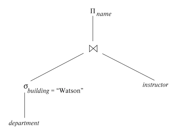 Figure 15.11 · PDF p. 753 · department selection, instructor join, name projection으로 구성된 operator tree
예를 들어 pi_name(sigma_building="Watson"(department) ⋈ instructor)는 먼저 department에 selection을 적용해 temporary relation을 만들고, 이를 instructor와 join한 뒤, 마지막에 projection을 수행한다.
Materialized evaluation cost는 개별 operation cost의 단순 합이 아니다. 앞의 operation cost estimates는 보통 operation result를 disk에 쓰는 비용을 제외했기 때문이다. Expression evaluation에서는 intermediate result를 temporary relation으로 쓰고 다시 읽는 비용이 들어간다.
Intermediate result r의 tuple 수가 nr, blocking factor가 fr이면 result block 수는 대략 nr / fr로 추정한다. Output buffer 크기가 bb blocks이면 temporary result write에 필요한 seeks는 대략 ceil(br / bb)로 볼 수 있다. double buffering은 두 buffers를 번갈아 사용해 한 buffer를 disk에 쓰는 동안 다른 buffer로 CPU processing을 계속하게 하므로 CPU와 I/O를 overlap할 수 있다.
15.7.2 Pipelining
pipelined evaluation은 intermediate temporary file을 줄이기 위해 여러 operations를 동시에 실행한다. 한 operation이 tuple을 생성하면 그 tuple을 바로 parent operation에 넘긴다. 예를 들어 pi_a1,a2(r ⋈ s)에서 join result를 temporary relation으로 쓰지 않고, join이 tuple을 하나 만들 때마다 projection으로 넘기면 intermediate write/read를 피한다.
Pipelining의 이득은 두 가지다.
| 이득 | 설명 |
|---|---|
| temporary I/O 제거 | intermediate relation을 disk에 쓰고 다시 읽는 비용을 줄인다. |
| early result | root operator까지 pipeline이 이어지면 query result를 생성되는 즉시 사용자에게 보여줄 수 있다. |
15.7.2.1 Implementation of Pipelining
Pipeline 구현 방식은 demand-driven pipeline과 producer-driven pipeline으로 나뉜다.
| 방식 | 별칭 | 동작 | 장점/용도 |
|---|---|---|---|
demand-driven pipeline | lazy, pulling | parent가 child에게 next tuple을 요청한다 | 구현이 쉽고 iterator model과 잘 맞음 |
producer-driven pipeline | eager, pushing | child operators가 tuples를 생성해 buffer에 밀어 넣는다 | parallel processing, code generation, CPU 효율에 유리 |
Demand-driven pipeline은 각 operator를 iterator로 구현한다. Iterator는 보통 open(), next(), close() interface를 가진다.
open()  -> operator 초기화
next()  -> 다음 output tuple 반환. 내부적으로 child.next()를 호출할 수 있음
close() -> 더 이상 tuple이 필요 없음을 알리고 자원 정리
Selection iterator의 open()은 file scan을 시작하고, next()는 이전 scan 위치 이후부터 계속 scan하여 다음 matching tuple을 반환한다. Merge-join iterator는 input iterators를 열고, 필요하면 input sort를 수행하며, next() 호출마다 다음 matching tuple pair를 반환한다. Iterator는 successive next() 호출 사이에 scan 위치, buffer 상태, current group 같은 execution state를 유지해야 한다.
Producer-driven pipeline은 adjacent operators 사이에 tuple buffer를 둔다. 각 operator는 별도 process/thread처럼 동작하며, output buffer가 찰 때까지 tuples를 생성하고, parent가 buffer를 비우면 다시 생성한다. Input buffer가 비어 있으면 lower operator가 더 생산할 때까지 기다린다. 이는 data를 아래에서 위로 pushing하는 방식이고, demand-driven은 위에서 아래로 pulling하는 방식이다.
Producer-driven은 modern CPU에서 function call overhead와 instruction cache miss를 줄일 수 있어 code generation 기반 high-performance query evaluation에서 점점 중요해진다. 반면 demand-driven은 구현이 단순해 전통적 DBMS iterator model에서 널리 쓰인다.
15.7.2.2 Evaluation Algorithms for Pipelining
Query plan의 edges는 pipelined edge와 blocking edge 또는 materialized edge로 나눌 수 있다. Pipelined edge로 연결된 operators는 producer/consumer 관계로 동시에 실행되어야 한다. Pipelined edges만으로 연결된 operator subtree를 pipeline stage라고 하며, query processor는 pipeline stage 단위로 실행을 조율한다.
blocking operator는 input을 모두 보거나 큰 단계를 끝내기 전에는 output을 낼 수 없는 operator다. Sorting은 대표적인 blocking operation이다. 하지만 sort 전체가 완전히 pipeline 불가능한 것은 아니다. External sort-merge는 run generation과 merge step으로 나눌 수 있고, run generation은 input과 pipelined될 수 있으며, merge step은 output consumer와 pipelined될 수 있다. Blocking은 두 sub-operators 사이, 즉 run generation이 끝나야 merge가 시작되는 지점에 존재한다.
Hash join도 비슷하게 나눌 수 있다. 일반 hash join은 양쪽 input을 partition한 뒤 build-probe를 시작하므로 전체적으로 blocking처럼 보인다. 하지만 sub-operator 관점에서는 relation scans에서 partition operators까지는 pipelined될 수 있고, build-probe output은 consumer에게 pipelined될 수 있다. Partition operators와 build-probe operator 사이가 blocking edge다.
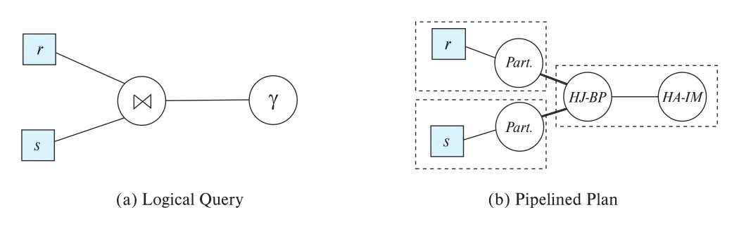 Figure 15.12 · PDF p. 758 · hash join을 partition/build-probe suboperators로 나누고 aggregation과 pipeline stage를 구성한 plan
Materialized edge마다 data를 disk에 쓰는 cost와 consumer가 다시 읽는 cost를 더해야 한다. 단, run generation과 merge처럼 단일 operator 내부 suboperators 사이의 materialization cost는 이미 해당 operator cost에 포함되어 있으므로 중복으로 더하면 안 된다.
double-pipelined join은 양쪽 input과 output 모두에 대해 pipeline을 유지하려는 기법이다. 두 input streams에서 tuple이 도착하는 대로 queue에 넣고, tuple이 r에서 왔으면 지금까지 받은 s tuples와 join하고, tuple이 s에서 왔으면 지금까지 받은 r tuples와 join한다. 이를 효율적으로 하려면 도착한 r, s tuples에 대해 index를 유지해야 한다. Hash indices를 쓰면 double-pipelined hash join이 된다.
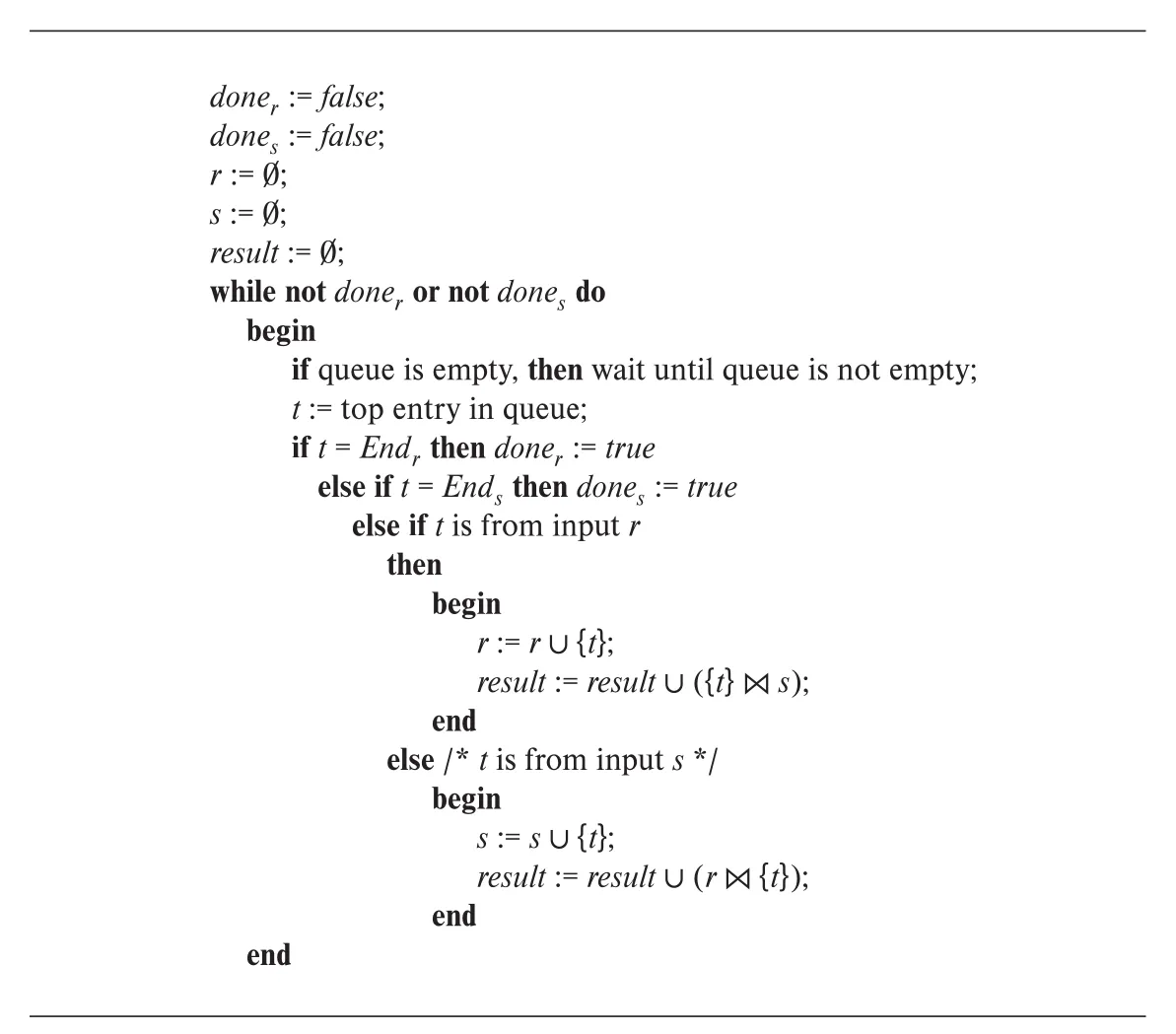 Figure 15.13 · PDF p. 759 · 두 input stream에서 도착하는 tuples를 queue로 받아 즉시 반대편 tuples와 join하는 double-pipelined join
Double-pipelined join은 두 inputs가 memory에 fit한다고 가정하면 가장 자연스럽다. Memory가 꽉 차면 지금까지 받은 tuples를 r0, s0 partition으로 보고 memory-resident index를 유지하며, 이후 tuples는 r1, s1 partition으로 disk에 쓰되 쓰기 전에 s0, r0와 probe한다. 마지막에는 r1과 s1을 기존 join technique으로 처리해야 전체 join이 완성된다.
15.7.3 Pipelines for Continuous-Stream Data
data streams처럼 tuples가 계속 들어오는 환경에서는 pipeline이 특히 중요하다. Stream 위의 query는 continuous query라고 하며, data가 도착하는 즉시 결과를 내야 하므로 blocking을 피하는 pipelined algorithms가 필요하다. 이 경우에는 producer-driven pipeline이 적합하다.
Continuous query에서는 windowing을 동반한 aggregation이 흔하다. tumbling window는 시간을 1분, 1시간처럼 고정 구간으로 나누고 각 window마다 grouping/aggregation을 수행한다. Memory가 충분하면 window별 group state를 in-memory hash index로 유지한다.
Window aggregate result는 해당 window에 더 이상 tuple이 오지 않는다는 사실을 알아야 output할 수 있다. Tuples가 timestamp order로 도착한다면 다음 window tuple의 도착이 이전 window 종료를 알려 준다. Out-of-order arrival이 가능하면 stream이 punctuation을 포함해 “이 시점 이하 timestamp의 tuple은 더 이상 오지 않는다”는 정보를 전달해야 한다.
15.8 Query Processing in Memory
지금까지의 algorithms는 주로 I/O cost를 줄이는 데 초점을 맞췄다. Data가 memory-resident이거나 SSD/main-memory 환경에서는 CPU cost, cache miss, function call overhead, data layout이 query processing 성능을 좌우한다.
15.8.1 Cache-Conscious Algorithms
Memory access는 disk/SSD보다 빠르지만, CPU cache에 이미 있는 data는 main memory보다 훨씬 빠르다. Modern CPU는 L1/L2/L3 cache를 가지며, main memory와 cache 사이 data transfer는 보통 cache line 단위로 일어난다. DBMS가 disk buffer처럼 CPU cache 내용을 직접 제어할 수는 없지만, algorithm과 layout을 cache-friendly하게 설계할 수 있다.
대표 cache-conscious ideas는 다음과 같다.
| 대상 | cache-conscious 설계 |
|---|---|
| in-memory sorting | run size를 cache에 fit하도록 정하고, 각 run을 cache 안에서 sort한 뒤 sequential merge |
| large external sorting | 큰 memory run 내부 sort에 cache-friendly in-memory merge-sort를 사용 |
| hash join | build relation partition과 hash index가 cache에 fit하도록 더 작은 partitions로 나누어 probe 시 cache misses를 줄임 |
| tuple layout | 함께 접근되는 attributes를 consecutive하게 배치해 한 cache line fetch로 필요한 값을 같이 가져옴 |
Cache miss가 발생하면 CPU core가 memory fetch를 기다리며 stall된다. OS와 DBMS는 multiple threads를 활용해 한 thread가 stall될 때 다른 thread가 실행되게 할 수 있고, 이는 Chapter 22의 parallel query processing으로 이어진다.
15.8.2 Query Compilation
Memory-resident data에서는 interpretation overhead도 커진다. 전통적 query execution engine은 plan을 해석하면서 relation metadata를 반복 조회하고, 각 record마다 function calls를 많이 수행한다. 예를 들어 attribute offset을 매번 metadata에서 찾는 것은 disk I/O가 지배적인 환경에서는 작은 비용일 수 있지만, main-memory DB에서는 병목이 된다.
query compilation은 query plan을 machine code 또는 intermediate byte-code로 compile해 이런 overhead를 줄인다. Compiler는 attribute offset을 compile time constant로 만들 수 있고, 여러 functions를 inline/merge해 function call 수를 줄일 수 있다. 원문은 compiled code가 interpreted execution보다 최대 한 자릿수 배율, 예를 들어 10배까지 빨라질 수 있다고 설명한다.
15.8.3 Column-Oriented Storage
column-oriented storage는 analytical query에서 필요한 attributes가 schema의 일부일 때 유리하다. Row store는 tuple 전체를 가져오므로 필요 없는 attributes까지 읽을 수 있지만, column store는 selection이나 aggregation에 필요한 columns만 읽을 수 있다. 반대로 많은 attributes를 함께 retrieve해야 하면 각 attribute마다 별도 access가 필요해 비용이 커질 수 있고, disk-resident data에서는 추가 seeks가 발생할 수 있다.
Column store는 vector processing과 잘 맞는다. 같은 attribute의 많은 values가 연속적으로 저장되므로, modern processor의 SIMD/vector instructions를 사용해 comparisons나 aggregations를 여러 values에 대해 병렬로 수행할 수 있다. Query compilation은 이런 vector-processing instructions를 생성해 CPU 효율을 높일 수 있다.
15.9 Summary
- Query processing은 SQL query를 internal form으로 변환하고, equivalent한 여러 방법 중 효율적인 plan을 골라 실행하는 과정이다.
- Simple selection은
linear scan또는 index를 사용한index scan으로 처리한다. Complex selection은 simple selection 결과의 union/intersection 또는 composite index, pointer intersection으로 처리할 수 있다. - Large relation sorting은
external sort-merge로 처리하며, run generation과 merge passes, available memoryM, per-run bufferbb가 cost를 결정한다. - Natural join/equi-join은
nested-loop join,block nested-loop join,indexed nested-loop join,merge join,hash join등으로 처리할 수 있고, index availability, input sortedness, memory size, cardinality가 선택 기준이다. - Duplicate elimination, projection, set operations, aggregation은 sorting 또는 hashing으로 구현할 수 있다.
- Outer join은 기존 join algorithm을 확장하거나 join 결과에 unmatched tuples를 null padding해 추가하는 방식으로 구현한다.
- Hashing과 sorting은 dual이다. Duplicate elimination, projection, aggregation, join, outer join처럼 hashing으로 구현 가능한 operation은 대체로 sorting으로도 구현 가능하고, 반대도 성립한다.
- Expression evaluation은
materialization또는pipelining으로 수행된다. Materialization은 단순하지만 temporary relation I/O가 크고, pipelining은 intermediate I/O를 줄이지만 blocking edge와 pipeline stage 관리가 필요하다. - In-memory query processing에서는 I/O보다 cache miss, CPU execution, interpretation overhead, column/vector processing이 중요해진다.
Review Terms 관점에서 검색성을 위해 남겨 둘 핵심 용어는 다음과 같다.
| 묶음 | 핵심 용어 |
|---|---|
| plan/cost | query processing, evaluation primitive, query-execution plan, query-evaluation plan, query-execution engine, measures of query cost, sequential I/O, random I/O |
| selection/sorting | file scan, linear search, access path, index scan, conjunctive selection, disjunctive selection, composite index, intersection of identifiers, external sorting, external sort-merge, runs, N-way merge |
| join | equi-join, nested-loop join, block nested-loop join, indexed nested-loop join, merge join, sort-merge join, hybrid merge join, hash join, build, probe, build input, probe input, recursive partitioning, hash-table overflow, skew, fudge factor, overflow resolution, overflow avoidance, hybrid hash join, spatial join |
| expression evaluation | operator tree, materialized evaluation, double buffering, pipelined evaluation, demand-driven pipeline, producer-driven pipeline, iterator, pipeline stage, double-pipelined join, continuous query evaluation |
| in-memory | cache-conscious algorithms, cache line, query compilation, column-oriented storage, vector processing |
Practice Exercises와 Exercises는 sort-merge pass 계산, join algorithm cost 비교, secondary index가 indexed nested-loop join에서 비효율적인 이유, iterator pseudocode, semijoin/anti-semijoin, demand-driven vs producer-driven pipelining, keyword query intersection, column-oriented storage의 장단점, hybrid merge/hash join 변형을 묻는다. 이 장을 이해했다면 “같은 relational operation을 어떤 physical algorithm으로 실행할 것인가”를 cost model, memory, index, sortedness, pipelining까지 포함해 설명할 수 있어야 한다.
연결 관계
- Chapter 14 Indexing: selection과 indexed nested-loop join은 B+ tree, secondary index, clustering index, bitmap index scan, spatial index 같은 access path 위에서 동작한다.
- Chapter 16 Query Optimization: Chapter 15의 algorithms와 cost estimates가 optimizer가 plan을 선택하는 입력이 된다.
- Chapter 13 Data Storage Structures: block 수
br, blocking factorfr, buffer sizeM, record layout, column-oriented storage가 query processing cost를 결정한다. - Chapter 22 Parallel and Distributed Query Processing: producer-driven pipeline, SSD parallel requests, multi-threading, data partitioning, distributed communication cost가 확장된다.
- Chapter 10 Big Data / stream data: continuous query, data streams, tumbling window, punctuation 기반 processing으로 연결된다.
오해하기 쉬운 내용
query-evaluation plan은 relational-algebra expression 자체가 아니다. 어떤 algorithm과 access path를 쓸지까지 포함한 physical plan이다.- Response time이 항상 optimizer의 직접 목표는 아니다. Buffer 상태와 parallel I/O에 크게 의존하므로 보통 total resource consumption을 근사해 최소화한다.
- Secondary index scan은 항상 빠르지 않다. Matching records가 많으면 record마다 random I/O가 생겨 linear scan보다 느릴 수 있다.
bitmap index scan은 Chapter 14의 bitmap index와 같은 말이 아니다. Secondary index 결과를 block bitmap으로 모아 block-order scan을 하는 hybrid access method다.- Index로 sorted order를 읽는 것과 records가 physical sorted order로 저장된 것은 다르다. Secondary index를 따라가면 tuple마다 random fetch가 생길 수 있다.
- Nested-loop join은 느리지만 가장 일반적이다. Equi-join이 아닌 complex join condition에도 사용할 수 있다.
- Hash join은 equality 기반 join에 강하지만, overlap/containment 같은 spatial predicate에는 직접 맞지 않는다.
- Merge join은 input이 이미 sorted되어 있으면 매우 싸지만, sorted되어 있지 않으면 sorting cost를 반드시 더해야 한다.
- Pipelining은 모든 operator를 무조건 streaming으로 만든다는 뜻이 아니다. Sorting, hash join처럼 blocking edge를 갖는 operator가 있다.
- Column store는 모든 query에 좋은 것이 아니다. 많은 attributes를 한 tuple 단위로 자주 읽으면 row store가 더 나을 수 있다.
면접 질문
query processing의 parsing/translation, optimization, evaluation 단계가 각각 무엇을 하는지 설명하라.evaluation primitive와query-evaluation plan이 relational-algebra expression과 어떻게 다른가?- Query cost model
b * tT + S * tS에서b,S,tT,tS의 의미와 SSD/main-memory에서 달라지는 점을 설명하라. - Linear search가 느려도 selection algorithm의 기본 fallback으로 필요한 이유는 무엇인가?
- Clustering index와 secondary index가 selection cost에 미치는 차이를 설명하라.
- PostgreSQL의
bitmap index scan이 secondary index scan과 linear scan 사이에서 어떤 절충을 제공하는지 설명하라. - External sort-merge의 run generation, merge pass,
M,bb,N-way merge를 설명하라. - Nested-loop join, block nested-loop join, indexed nested-loop join의 적용 조건과 cost 차이를 비교하라.
- Merge join이 input sortedness에 의존하는 이유와, unsorted input에서 sort cost를 더해야 하는 이유를 설명하라.
- Hash join의 build input/probe input, partitioning, build-probe phase를 설명하라.
- Hash join에서 skew와 hash-table overflow가 왜 문제이며, overflow resolution/avoidance가 어떻게 다른지 설명하라.
- Hybrid hash join이 어떤 상황에서 일반 hash join보다 비용을 줄이는지 설명하라.
- Duplicate elimination, projection, set operations, aggregation이 sorting 또는 hashing으로 구현되는 공통 원리를 설명하라.
- Materialized evaluation과 pipelined evaluation의 장단점을 temporary relation I/O 관점에서 비교하라.
- Demand-driven pipeline과 producer-driven pipeline의 차이를 iterator model, buffering, parallelism 관점에서 설명하라.
- Blocking edge와 pipeline stage가 무엇이며, sort와 hash join이 왜 sub-operators로 나뉠 수 있는지 설명하라.
- Continuous query에서 windowing과 punctuation이 필요한 이유를 설명하라.
- In-memory query processing에서 cache-conscious algorithm과 query compilation이 중요한 이유를 설명하라.
- Column-oriented storage가 analytical query와 vector processing에 유리한 이유와, row retrieval에는 불리할 수 있는 이유를 설명하라.
- Chapter 15의 query processing algorithms가 Chapter 16 query optimization에서 어떻게 사용되는지 설명하라.