개요
Chapter 21은 Chapter 20의 architecture 논의를 실제 storage 설계로 내린다. Parallelism은 query를 더 빨리 실행하는 speedup과 workload 증가를 response time 증가 없이 흡수하는 scaleup을 제공하지만, 이를 얻으려면 data 자체가 여러 node에 어떻게 놓이는지 결정해야 한다.
이 장의 중심은 shared-nothing parallel database에서 relation을 여러 node로 나누는 data partitioning, partitioning이 만들 수 있는 skew, failure와 availability를 위한 replication, 여러 node 위의 parallel indexing, 대규모 file을 저장하는 distributed file system, 그리고 nonrelational data를 key로 저장하는 parallel key-value store다. 이 기법들은 parallel database뿐 아니라 geographically distributed database에도 적용된다.
핵심 개념
horizontal partitioning은 relation의 tuples를 여러 node에 나누어 각 tuple이 한 node에 있도록 하는 방식이다.- 기본 partitioning strategy는
round-robin partitioning,hash partitioning,range partitioning이다. - Access pattern이
scan,point query,range query인지에 따라 좋은 partitioning strategy가 달라진다. skew는 tuple 또는 workload가 특정 partition/node에 몰려 parallelism을 망가뜨리는 현상이다.- Small relation은 무작정 partitioning하지 않는 편이 낫다. 각 node에 몇 tuple만 남으면 parallelism보다 overhead가 커진다.
세부 정리
21.1 Overview
Parallel/distributed storage의 첫 질문은 “data를 여러 node에 어떻게 나눌 것인가”다. Section 21.2와 21.3은 data partitioning과 skew를 다루고, Section 21.4는 availability를 위한 replication을, Section 21.5는 partitioned data 위의 indexing을 다룬다. Section 21.6의 distributed file system은 많은 node 위에서 file을 저장하는 일반적 방법이고, Section 21.7의 parallel key-value store는 unstructured text, XML, JSON 같은 nonrelational/semi-structured data를 key와 함께 저장하는 구조다.
이 장에서 data storage system은 두 의미를 함께 포괄한다.
| 용어 | 이 장에서의 의미 |
|---|---|
| parallel database의 storage/access layer | relational tuples를 여러 node에 partition/replicate/index하는 계층 |
| parallel key-value store | key가 붙은 data item을 여러 node에 저장하고 접근하는 system |
Query processing은 Chapter 22, transaction processing은 Chapter 23에서 자세히 다룬다. Chapter 21은 그 둘이 올라탈 storage layout을 만든다.
21.2 Data Partitioning
가장 단순한 I/O parallelism은 data를 여러 disks에 나누어 저장해 disk에서 data를 가져오는 시간을 줄이는 것이다. RAID는 block을 여러 disks에 round-robin으로 배치해 parallel access를 가능하게 한다. 예를 들어 n개의 disk가 있으면 block i를 disk i mod n에 배치할 수 있다.
하지만 RAID의 block-level partitioning은 어떤 tuple이 어떤 disk/node에 저장되는지를 DBMS가 제어하지 못한다. Parallel database system은 보통 block이 아니라 tuple level에서 partitioning한다. 여러 node가 있고 각 node가 여러 disk를 가진다면, DBMS는 data를 node들 사이에 나누고, node 내부 disk 배치는 OS 또는 local storage layer에 맡긴다.
horizontal partitioning은 relation의 tuples를 여러 node에 나누어 각 tuple이 정확히 한 node에 저장되게 하는 방식이다. 반면 vertical partitioning은 relation의 attributes를 나누는 방식이다. 예를 들어 r(A, B, C, D)에서 A가 primary key이고 B는 자주 필요하지만 C, D가 크고 자주 필요하지 않다면 r(A, B)와 r(A, C, D)로 vertical partitioning할 수 있다. Horizontal partitioning 후 각 node 안에서 vertical partitioning을 함께 사용할 수도 있다.
주의할 점은 vendor가 partitioning이라는 말을 single node 안에서 relation r을 physical relations r1, r2, ..., rn으로 나누는 의미로 쓰기도 한다는 점이다. 이 장에서는 이후 특별히 말하지 않으면 multiple nodes across horizontal partitioning을 뜻한다.
21.2.1 Partitioning Strategies
Relation tuples를 n개 node N1, N2, ..., Nn에 나누는 기본 전략은 세 가지다.
| Strategy | 배치 방식 | 강점 | 약점 |
|---|---|---|---|
round-robin partitioning | scan 순서의 i번째 tuple을 N((i-1) mod n)+1에 보낸다. | tuple 수가 node별로 거의 균등하다. Full scan에 좋다. | point query/range query는 모든 node를 찾아야 한다. |
hash partitioning | partitioning attributes에 hash function을 적용해 결과 node에 tuple을 둔다. | partitioning attribute에 대한 point query가 빠르다. Key hash가 좋으면 균등 분포가 쉽다. | nonpartitioning attribute query와 range query에는 약하다. |
range partitioning | partitioning attribute의 contiguous value range를 node별로 할당한다. | partitioning attribute의 point query와 range query에 좋다. | 특정 range에 data/query가 몰리면 hot spot과 execution skew가 생긴다. |
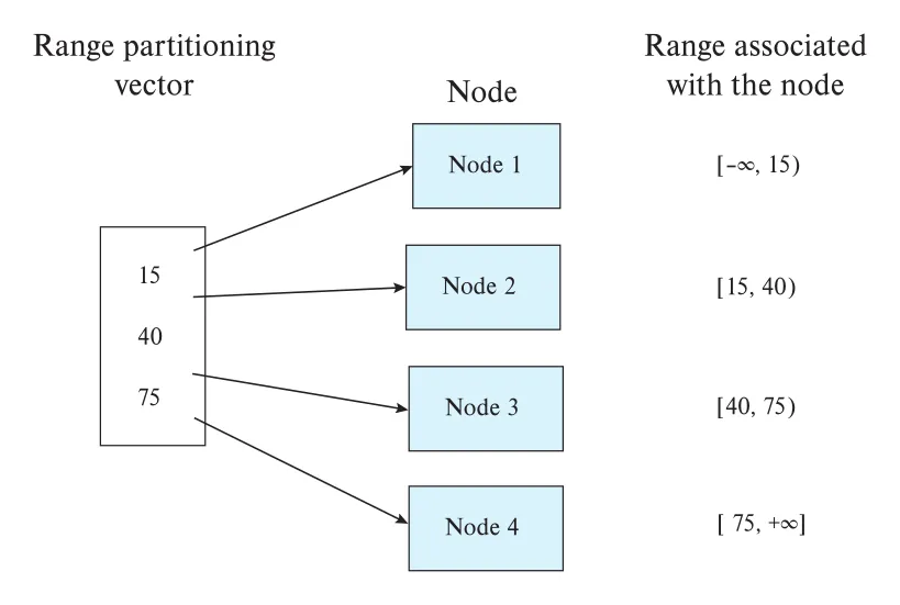 Figure 21.1 · PDF p. 1034 · partitioning vector로 attribute value range를 node에 매핑하는 예
Figure 21.1은 range partitioning vector의 의미를 보여준다. Partitioning attribute A에 대해 vector [15, 40, 75]가 있으면, x < 15는 Node 1, 15 <= x < 40은 Node 2, 40 <= x < 75는 Node 3, x >= 75는 Node 4로 간다. Range boundary는 query routing과 tuple placement를 동시에 결정한다.
Update 시 partitioning 유지 방식도 strategy에 따라 달라진다.
| Operation | 처리 방식 |
|---|---|
| Insert | partitioning strategy에 따라 appropriate node로 tuple을 보낸다. |
| Delete | partitioning attribute 값으로 위치를 찾은 뒤 삭제한다. Round-robin에서는 모든 partition을 검색해야 할 수 있다. |
| Update | partitioning attribute가 변하지 않으면 제자리 update가 가능하다. Hash/range partitioning에서 partitioning attribute가 바뀌면 old location에서 delete하고 new location에 insert해야 한다. |
21.2.2 Comparison of Partitioning Techniques
Partitioned relation은 여러 node에서 parallel하게 read/write할 수 있어 전체 relation scan이나 relation loading의 transfer rate가 높아진다. 하지만 모든 access가 full scan은 아니다. Data access pattern은 크게 세 종류로 나뉜다.
| Access pattern | 의미 |
|---|---|
scan | entire relation을 순차적으로 읽는다. |
point query | 특정 attribute가 특정 value인 tuple을 찾는다. 예: employee name = "Campbell" |
range query | 특정 attribute value가 주어진 range 안에 있는 모든 tuple을 찾는다. 예: 10000 < salary < 20000 |
Partitioning technique별 효율은 다음과 같다.
| Technique | Scan | Point query | Range query |
|---|---|---|---|
round-robin | 모든 node가 거의 같은 양을 읽어 full scan에 이상적이다. | 모든 node를 search해야 한다. | 모든 node를 search해야 한다. |
hash partitioning | 좋은 hash function과 key partitioning attribute라면 node별 tuple 수가 거의 같아 1/n scan time에 가깝다. | partitioning attribute의 point query는 hash로 target node 하나만 찾으면 된다. | hash가 value proximity를 보존하지 않으므로 대개 모든 node를 scan해야 한다. |
range partitioning | range가 균등하면 scan도 병렬 가능하다. | partitioning vector로 target node를 찾을 수 있다. | partitioning vector로 관련 node range만 찾을 수 있다. |
Hash partitioning의 큰 장점은 partitioning attribute point query에서 start-up cost를 줄인다는 점이다. Query를 모든 node에 시작하지 않고 한 node로 보내면 다른 nodes는 다른 query를 처리할 수 있어 throughput이 올라간다.
Range partitioning은 range query가 작은 범위일 때 특히 좋다. 관련 node만 검색하면 되므로 response time과 throughput을 함께 유지할 수 있다. 그러나 query range가 domain의 큰 부분을 차지하거나 data가 특정 range에 몰리면, 몇 node에 I/O bottleneck 또는 hot spot이 생긴다. 이런 상황은 Section 21.3의 execution skew로 이어진다. 반면 hash/round-robin은 range query에서 모든 node를 사용하므로 같은 throughput에서 response time이 더 좋을 수도 있다.
결론적으로 선택은 operation mix에 따라 다르다. 일반적으로 round-robin보다 hash partitioning 또는 range partitioning이 선호된다. 다만 partitioning은 large relation에 의미가 크다. Small relation을 모든 node에 나누면 node마다 몇 tuple만 남아 overhead가 커지므로, small relation은 unpartitioned로 두고 medium-sized relation은 large system의 일부 node에만 partitioning하는 편이 낫다.
21.3 Dealing with Skew in Partitioning
skew는 parallel storage에서 자주 성능을 무너뜨리는 문제다. Round-robin이 아닌 partitioning에서는 일부 partition에 tuple이 많이 들어가고 다른 partition은 적게 들어가는 불균형이 생길 수 있다. Tuple distribution 자체가 불균형인 경우를 data distribution skew라고 한다.
Data distribution skew는 두 원인으로 나눌 수 있다.
| Skew 종류 | 원인 | 예/결과 |
|---|---|---|
attribute-value skew | partitioning attribute의 특정 값이 많은 tuples에 반복된다. | 같은 partitioning value를 가진 tuples가 모두 같은 partition으로 가므로 hash/range 모두 skew가 생길 수 있다. |
partition skew | attribute-value skew가 없어도 partitioning boundary/hash choice 때문에 load가 불균등하다. | range partitioning vector를 잘못 고르면 특정 range가 너무 커진다. 좋은 hash function이면 hash partitioning에서는 덜 생긴다. |
Skew는 parallelism이 커질수록 더 위험해진다. 1000 tuples를 10 partitions로 나눌 때 평균은 100이지만 한 partition이 200이면 실제 speedup은 10이 아니라 5 수준으로 떨어진다. 100 partitions로 나누면 평균은 10인데 한 partition이 40이어도 speedup은 100이 아니라 25 수준이 된다. Parallel task의 completion time은 결국 가장 느린 partition/node가 결정하기 때문이다.
execution skew는 tuple 수가 균등해도 query access가 특정 partition에 몰리는 현상이다. 예를 들어 timestamp로 partitioning했는데 대부분의 query가 recent tuples만 조회하면, recent timestamp range를 가진 partition이 훨씬 높은 load를 받는다.
21.3.1 Balanced Range-Partitioning Vectors
Range partitioning의 data distribution skew는 balanced range-partitioning vector를 고르면 줄일 수 있다. 가장 직접적인 방법은 relation을 partitioning attributes로 sort하고, sorted order로 scan하면서 relation의 1/n마다 다음 tuple의 partitioning attribute value를 partition vector에 넣는 것이다. 이렇게 하면 n개 partition에 tuple이 거의 균등하게 들어간다.
단점은 initial sort의 extra I/O overhead가 크다는 점이다. 이 비용은 attribute value의 frequency table 또는 histogram을 사용해 줄일 수 있다.
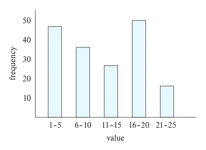 Figure 21.2 · PDF p. 1038 · integer-valued attribute의 value range별 frequency histogram 예
Figure 21.2 같은 histogram이 있으면 value distribution을 보고 balanced range-partitioning function을 만들 수 있다. Histogram은 system catalog에 여러 attribute별로 저장할 수 있을 만큼 작다. 저장된 histogram이 없으면 relation의 random disk blocks에서 sampling해 approximate histogram을 만들 수 있고, 이는 full sort보다 훨씬 빠르다.
이 방식은 data-distribution skew에는 도움이 되지만 static하다. Partitioning vector를 한 번 정한 뒤 insert/delete/update가 계속되면 skew가 다시 생길 수 있다. Skew를 감지할 때마다 vector를 다시 계산하고 data를 repartition할 수 있지만, large data에서는 expensive하고 normal processing에 큰 load를 준다. 그래서 더 동적인 방법으로 virtual node와 dynamic repartitioning을 사용한다.
21.3.2 Virtual Node Partitioning
virtual node partitioning은 real node보다 훨씬 많은 virtual nodes가 있다고 가정하고, tuple과 work를 먼저 virtual node에 매핑한 뒤 virtual node를 real node에 매핑하는 방식이다. Virtual node 방식은 virtual processor approach라고도 불렸지만, VM 문맥의 virtual processor와 혼동을 피하기 위해 여기서는 virtual node라고 한다.
가장 단순한 매핑은 virtual node를 real node에 round-robin으로 배정하는 것이다. Real nodes가 1..n이면 virtual node i를 real node ((i - 1) mod n) + 1에 배정한다. 어떤 range가 skew로 많은 tuples를 가져도 그 range가 여러 virtual node ranges로 쪼개지고, virtual nodes가 여러 real nodes에 퍼지면 한 real node에 부담이 몰리지 않는다.
더 정교한 방식은 각 virtual node의 tuple 수와 access load, 예를 들어 requests per second를 추적하고, real node별 stored tuples와 load가 균형이 되도록 virtual-to-real mapping을 조정하는 것이다. 이 방식은 data-distribution skew와 execution skew를 모두 줄일 수 있다.
System은 이 mapping을 기록해야 한다. Virtual node가 consecutive integers라면 virtual_to_real_map[] 같은 array로 저장할 수 있고, i번째 entry가 virtual node i가 올라간 real node를 가리킨다.
Virtual node의 또 다른 장점은 storage elasticity다. Load가 커져 new real node를 추가하면 일부 virtual nodes만 새 node로 migrate하면 된다. Virtual node마다 data 양이 작으면 migration이 빠르고, 다른 virtual nodes에 영향을 주지 않아 disruption이 작다.
21.3.3 Dynamic Repartitioning
Virtual node 방식도 data distribution이 시간에 따라 변하면 한계가 있다. Timestamp로 partitioning한 경우 새 records가 계속 최신 timestamp range에 들어가므로, 처음에는 balanced였던 virtual node도 시간이 지나면 overfull 또는 overloaded가 될 수 있다.
전체 partitioning scheme을 다시 계산하고 data를 모두 옮기는 것은 너무 비싸다. 대신 dynamic repartitioning은 overfull virtual node를 두 virtual nodes로 split한다. 이는 B+-tree node가 overfull일 때 split되는 것과 비슷하다. Split 후 새로 생긴 virtual node 중 하나를 다른 real node로 migrate하면 data 양이나 load를 다시 균형 있게 만들 수 있다.
Parallel data storage system에서는 data item collection을 table이라고 부르고, table을 여러 tablet으로 나눈다. Tablet은 virtual node에 해당하며, tablet 수는 real node 수보다 훨씬 많다.
System은 partition table을 유지한다. Partition table은 partitioning key ranges를 tablet identifier와 tablet data가 있는 real node에 매핑한다.
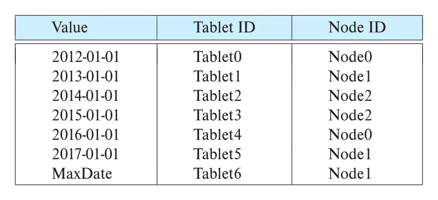 Figure 21.3 · PDF p. 1040 · date partition key range를 tablet과 real node에 매핑한 partition table 예
Read request는 partitioning attribute value를 제공해야 한다. System은 그 value가 속한 key range를 찾아 tablet을 결정하고, partition table에서 tablet이 있는 real node를 찾아 request를 보낸다. Partitioning attribute value가 없는 read request는 모든 tablets로 보내야 한다. 각 tablet에는 partitioning key attribute index를 유지하면 local lookup을 효율적으로 처리할 수 있다.
Write, insert, delete도 같은 방식으로 correct tablet과 real node로 routing된다. Tablet이 너무 커지면 tablet의 key range를 둘로 나누고, 새 tablet이 half key range를 갖는다. 해당 key range의 records를 original tablet에서 new tablet으로 옮긴 뒤 partition table을 갱신한다.
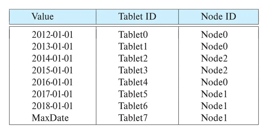 Figure 21.4 · PDF p. 1041 · Tablet6 split과 Tablet1 move 이후 partition table 변화
Figure 21.4는 Figure 21.3의 Tablet6이 2017-01-01 <= key < 2018-01-01과 2018-01-01 <= key로 split되고, Tablet1이 Node1에서 Node0으로 move된 예를 보여준다. Split은 tablet size를 줄이고, move는 real node의 data/load imbalance를 줄인다.
Partition table은 보통 master node에 저장된다. 하지만 초당 많은 requests를 처리하려면 partition table을 모든 client nodes 또는 여러 router에 replicate한다. Router는 client read/write request를 받아 key value를 보고 appropriate real node로 forward한다.
Master/router가 없는 fully distributed approach도 있다. consistent hashing은 keys와 node 또는 virtual node identifiers를 같은 large hash space, 예를 들어 32-bit integer space에 hash한다. Hash space를 circle처럼 보고, key hash에서 반시계 방향으로 가장 가까운 node hash에 key를 매핑한다. 이 아이디어를 사용한 distributed hash table(DHT)에서는 master나 router 없이 각 participating node가 몇 peer node를 알고 cooperative routing을 수행한다. New node도 protocol을 따라 peer-to-peer 방식으로 join할 수 있다.
21.4 Replication
Node 수가 많아질수록 system 전체에서 적어도 하나의 node가 실패할 확률은 커진다. 단일 node가 5년에 한 번 실패한다고 해도 100-node system에서는 평균적으로 약 18일마다 어떤 node failure가 생길 수 있다. 잘못 설계된 parallel system은 node 하나만 실패해도 멈출 수 있으므로, parallel data storage system은 node failure에 resilient해야 한다.
Replication의 목적은 두 가지다.
- Node failure가 발생해도 data를 잃지 않는다.
- Failure 중에도 system이 계속 function하여
availability를 유지한다.
Tuple 단위로 replica를 추적하면 storage와 query processing overhead가 크다. 따라서 replication은 보통 partitions, tablets, nodes, virtual nodes 수준에서 수행된다. 각 partition의 replicas 위치는 partition table에 기록된다.
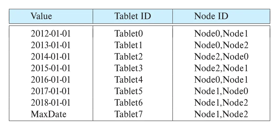 Figure 21.5 · PDF p. 1043 · Figure 21.4의 partition table에 tablet replica node 목록을 추가한 예
Figure 21.5는 각 tablet이 두 node에 replicate된 partition table을 보여준다. DBMS는 failed nodes를 추적하고, failed node에 있던 data request를 replica가 있는 backup node로 자동 route한다.
21.4.1 Location of Replicas
Two-way replication은 single node failure에 대비하고, three-way replication은 two node failures까지 대비할 수 있다. Low-cost commodity machines를 많이 쓰는 system은 보통 three-way replication을 사용하고, 더 reliable한 machines를 쓰는 system은 two-way replication을 사용할 수 있다.
Replica placement는 failure mode를 고려해야 한다.
| Failure mode | Placement 원칙 |
|---|---|
| single node failure | 다른 node에 replica를 둔다. |
| rack failure | same rack 내부 replication만으로는 부족하므로 다른 rack에도 replica를 둔다. |
| entire data center failure | geographically separated data centers에 replica를 둔다. |
Data center 내부에서는 rack 안 bandwidth가 rack 간 bandwidth보다 크므로 same rack replica는 network demand를 줄인다. 하지만 rack power/network switch failure를 견디려면 다른 rack에도 replica가 있어야 한다. Data center 전체 failure, 예를 들어 fire/flood/large-scale power failure를 견디려면 replication across data centers가 필요하다. 특히 web application에서는 user와 가까운 data center에 application server와 data replica를 배치해 long-distance round-trip delay를 줄인다.
Replica placement는 failure 중 execution skew도 고려해야 한다. Node N1의 모든 partitions가 단일 node N2에만 replicate되어 있으면 N1 failure 시 N2가 자기 원래 workload와 N1 workload를 모두 처리해 load가 두 배가 된다. 이를 피하려면 N1의 partitions replica를 여러 다른 nodes에 분산해 failure 시 extra work가 여러 nodes로 나뉘게 한다.
21.4.2 Updates and Consistency of Replicas
Partition이 replicate되면 update는 모든 replica에 반영되어야 한다. Data가 생성 후 never updated라면 어느 replica에서 읽어도 같은 값을 얻는다. 하지만 update가 있는 경우 replica update 방식에 따라 consistency가 달라진다.
가장 강한 방식은 모든 replicas에 exclusive lock을 걸고 atomic하게 update하는 것이다. 예를 들어 two-phase commit(2PC)를 사용하면 all replicas update가 atomic하게 적용되고, shared lock을 얻은 read는 어떤 replica에서 읽어도 most recent version을 볼 수 있다.
Replica가 atomic하게 update되지 않으면 temporarily different values가 생긴다. 이때 read가 어느 replica에 가느냐에 따라 다른 값을 볼 수 있고, older version을 읽고 update하면 lost update가 생길 수 있다.
이를 줄이는 한 방법은 각 partition replica 중 하나를 master replica로 지정하는 것이다. 모든 updates는 master replica로 보내고, master가 다른 replicas로 propagate한다. Reads도 master replica에서 수행하면, other replicas에 아직 update가 반영되지 않았더라도 latest version을 읽을 수 있다.
Master replica failure가 발생하면 new master를 assign해야 한다. 이때 old master가 수행한 모든 update operation을 new master가 알고 있어야 하고, old master가 일부 replicas만 update한 뒤 실패했다면 new master가 나머지 replica update를 완료해야 한다. Partition table은 key range, replica locations뿐 아니라 current master replica도 기록해야 한다.
Replica update에는 세 가지 대표 방법이 있다.
| 방법 | 일관성 특성 | 장단점 |
|---|---|---|
two-phase commit(2PC) | all replicas update를 atomic하게 적용 | 강한 consistency를 제공하지만 unreachable replica/failure 처리가 복잡하다. |
persistent messaging | update message가 eventually all replicas에 delivered됨 | eventual consistency를 제공한다. 중간에는 replicas가 다른 값을 가질 수 있어 reads를 master에 보내는 방식이 필요하다. |
consensus protocols | 일부 replica가 unreachable이어도 replica updates를 진행할 수 있음 | designated master 없이도 동작할 수 있으며, Chapter 23.8의 distributed consensus로 이어진다. |
21.5 Parallel Indexing
Parallel data storage system의 indices는 local index와 global index로 나뉜다. Virtual node partitioning을 사용할 때 여기서 node는 virtual node 또는 tablet으로 이해하면 된다.
| Index 종류 | 정의 | 저장 위치/용도 |
|---|---|---|
local index | 특정 node에 저장된 tuples 위에 만든 index | index contents가 data와 같은 node에 있다. 각 partition의 local lookup에 좋다. |
global index | 여러 node에 저장된 data 전체를 대상으로 matching tuples를 찾는 index | single central location에 두면 scalability가 나쁘므로 global index 자체도 multiple nodes에 partition해야 한다. |
global primary index는 relation이 partitioned된 attributes와 같은 attributes 위의 global index다. Partitioning attribute K에 global primary index를 만들려면 각 partition에 K local index를 만들면 된다. Query가 K = k1 같은 key value를 찾으면 partitioning function으로 k1이 있을 partition을 찾고, 그 partition의 local index로 tuple을 찾는다.
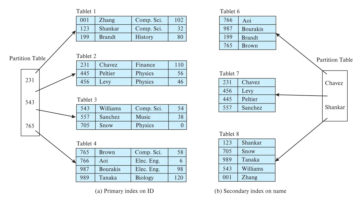 Figure 21.6 · PDF p. 1047 · student relation의 ID 기반 global primary index와 name 기반 global secondary index
Figure 21.6(a)는 student relation이 ID로 partitioned되어 있고, ID에 global primary index가 있는 경우다. ID = 557 query는 ID partitioning function으로 target tablet/node를 찾고 그 node의 local ID index를 사용한다. Partitioning scheme이 range-based라면 range query도 지원할 수 있지만, hash partitioning은 range query를 지원하기 어렵다.
global secondary index는 index attributes가 partitioning attributes와 다른 global index다. 예를 들어 student relation이 ID로 partitioned되어 있는데 name으로 search하고 싶으면, 각 partition에 local name index만 두는 방식은 모든 partitions에 query를 보내야 하므로 partition 수가 클수록 비효율적이다.
효율적인 global secondary index는 별도 relation처럼 만든다. 예를 들어 index_name(name, ID) tuples를 만들고, 이 index_name relation을 name으로 partition한다. 각 index_name partition에는 local name index를 만들고, base relation student에는 ID global index가 있다. name = Shankar query는 먼저 index_name의 partitioning function으로 name partition을 찾고, 그 local index에서 matching ID를 얻은 뒤, ID global index로 base tuple을 찾는다.
일반적으로 relation r이 partitioning attributes Kp로 partitioned되어 있고, secondary index attributes가 Ki라면, global secondary index relation ris는 다음 attributes를 포함한다.
Ki와KpKp에 duplicates가 있으면,Kp ∪ Ku가 original relation key가 되도록 추가 attributesKu
ris는 Ki로 partitioned되고 Ki local index를 가진다. Base relation r의 각 partition에는 (Kp, Ku) local index를 둔다. Query value v for Ki는 ris의 relevant partition에서 candidate (Kp, Ku) 값을 찾고, 그 값을 Kp 기준으로 repartition해 corresponding base relation nodes로 보내며, 각 node의 local (Kp, Ku) index로 matching tuples를 찾는다.
Global secondary index는 사실상 materialized view다.
따라서 base relation r에 insert/delete/update가 발생하면 ris도 함께 update되어야 한다. 이 update가 다른 nodes에 걸칠 수 있으므로, base relation update와 secondary index update를 같은 transaction으로 atomic commit하려면 2PC가 필요하다. Secondary index가 잠시 stale해도 되는 application이라면 persistent messaging 기반 asynchronous update도 가능하다.
21.6 Distributed File Systems
distributed file system은 files를 많은 machines에 나누어 저장하면서 client에게는 single-file-system view를 제공한다. Client는 file names와 directories로 file을 식별하고 접근하며, file이 실제로 어느 node에 저장되었는지는 신경 쓰지 않아도 된다.
초기 distributed file system은 client machines가 one or more file servers에 저장된 files를 접근하는 데 초점을 맞췄다. 이 장에서 다루는 later-generation distributed file system은 file blocks를 매우 많은 nodes에 분산해 저장한다. 대표적인 구조가 Google File System(GFS)이고, Hadoop File System(HDFS)은 GFS architecture를 바탕으로 널리 쓰인다.
Distributed file system과 parallel data storage system은 저장 대상의 크기와 개수가 다르다.
| System | 대상 | 설계 초점 |
|---|---|---|
distributed file system | tens of MB부터 hundreds of GB 이상인 large files, 보통 millions 수준의 file 수 | large sequential file storage/access, block partitioning, block replication |
parallel data storage system | tens of bytes부터 몇 MB까지의 data items, billions 이상 가능 | very large number of items, key-based access/update |
File은 data item보다 훨씬 클 수 있으므로 여러 block으로 쪼개고, 한 file의 blocks를 여러 machines에 partition한다. 각 file block은 machine failure로 file이 inaccessible해지는 것을 막기 위해 multiple machines, 보통 세 machines에 replicate된다.
File system metadata는 두 종류가 필요하다.
- Files를 directories/subdirectories로 조직하는 directory system.
- File name을 file data blocks의 block identifiers sequence로 매핑하는 정보.
Distributed file system에서는 block identifier만으로는 부족하다. Block이 어느 node에 저장되어 있는지도 알아야 하고, replication 때문에 각 block identifier마다 replica node identifiers set을 제공해야 한다.
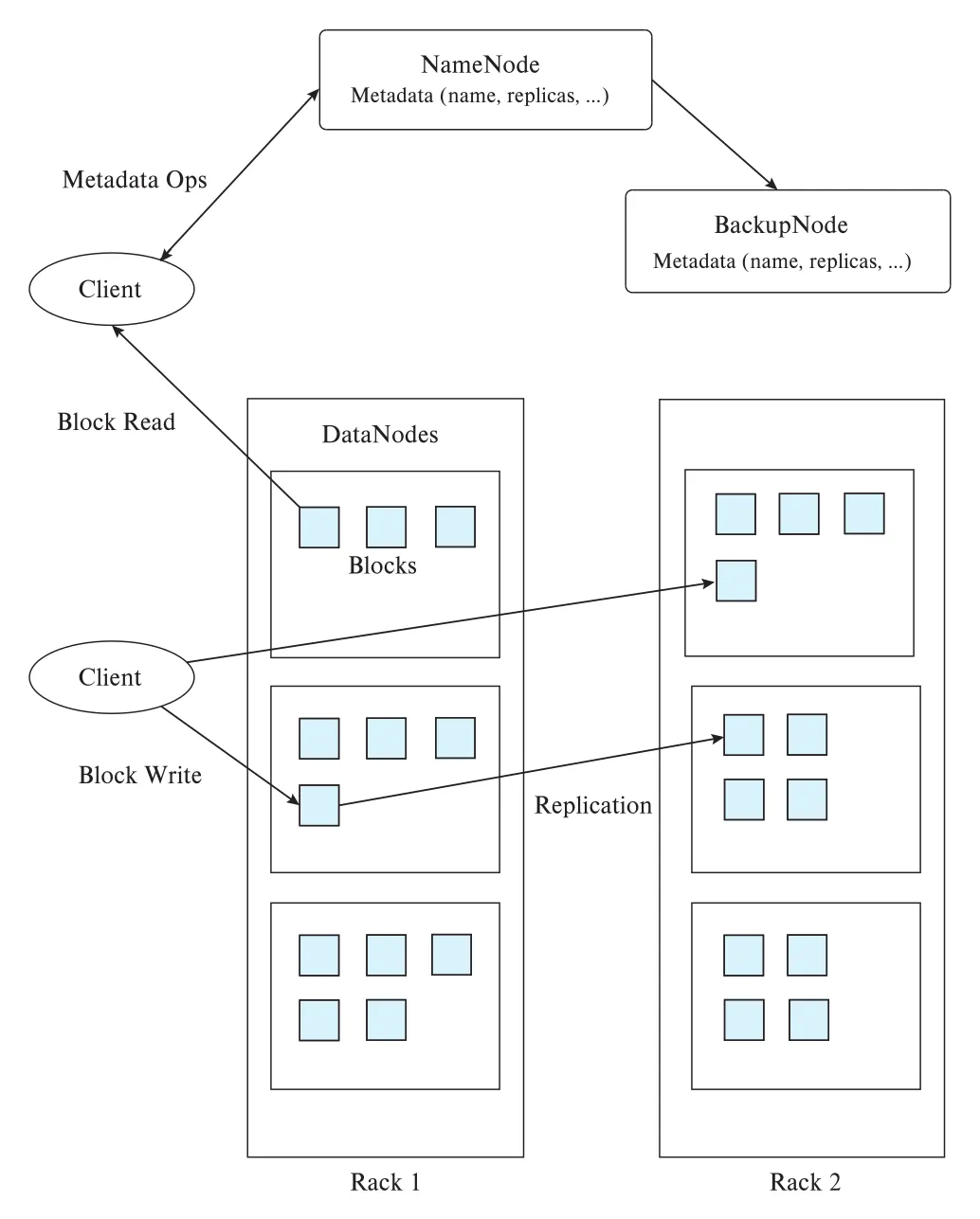 Figure 21.7 · PDF p. 1050 · NameNode, DataNodes, BackupNode로 구성된 HDFS architecture
Figure 21.7은 HDFS의 핵심 구조를 보여준다. HDFS에서 data blocks를 저장하는 machines는 datanodes다. 각 block은 block ID를 가지고, datanode는 block ID를 local file system의 실제 저장 위치에 매핑한다. Metadata는 단일 node인 namenode에 저장한다. Metadata를 여러 node에 partition할 수도 있지만 성능과 복잡성이 커지므로, GFS/HDFS는 pragmatic하게 single namenode 방식을 택했다.
Namenode는 모든 metadata reads를 처리하므로, metadata read마다 disk access가 필요하면 throughput이 너무 낮아진다. 그래서 HDFS namenode는 entire metadata를 memory에 cache한다. 이 때문에 namenode의 memory size가 manage 가능한 files/blocks 수를 제한한다. HDFS는 block size를 매우 크게, 보통 64 MB 정도로 잡아 file당 block 수를 줄이고 namenode metadata 부담을 낮춘다. 이 설계 덕분에 files 수는 millions 수준으로 제한될 수 있지만, total data size는 many petabytes까지 가능하다.
HDFS read 흐름은 다음과 같다.
| 단계 | 동작 |
|---|---|
| 1 | Client가 file name으로 namenode에 open/read metadata request를 보낸다. |
| 2 | Namenode가 file data를 담은 block IDs와 각 block replica를 가진 datanodes set을 반환한다. |
| 3 | Client가 각 block의 replica 중 하나에 직접 block ID를 보내 data block을 읽는다. |
| 4 | 선택한 replica가 응답하지 않으면 다른 replica에 요청한다. |
Write 흐름은 반대 방향으로 metadata allocation과 data block write가 분리된다.
| 단계 | 동작 |
|---|---|
| 1 | Client가 namenode에 write request를 보낸다. |
| 2 | Namenode가 blocks를 allocate하고, 각 block replica를 저장할 datanodes를 결정한다. |
| 3 | Metadata가 namenode에 기록되고 client에 반환된다. |
| 4 | Client가 block을 모든 replicas에 쓴다. 모든 replicas가 block write를 처리하면 acknowledgment가 client로 간다. |
Network traffic을 줄이기 위해 HDFS는 두 replicas를 같은 rack에 둘 수 있다. 이 경우 client가 한 replica에 block을 쓰고, 그 replica가 same rack의 두 번째 replica로 copy하는 방식이 가능하다. 이는 rack 내부 bandwidth가 rack 간 bandwidth보다 크다는 Chapter 20의 data-center topology 논의와 연결된다.
Replication은 replica consistency 문제를 만든다. 한 block replica만 update되고 다른 replica는 failure로 update되지 않으면, 어느 replica를 읽느냐에 따라 다른 값을 볼 수 있다. 일반 data storage system은 Chapter 23의 consistency technique으로 이를 다루지만, HDFS는 다른 접근을 택한다. 즉, written data를 update하지 못하게 하고 append만 허용한다.
HDFS의 file model은 write-once-read-many access model이다. File은 append될 수 있지만 이미 written data는 update되지 않는다. File은 close되기 전, 즉 모든 data가 write되고 blocks가 모든 replicas에 성공적으로 written되기 전에는 read할 수 없다. Updates가 필요한 application은 distributed file system보다 update-supporting data storage system을 사용해야 한다.
21.7 Parallel Key-Value Stores
대규모 Web application은 수십억 개 이상의 작은 records를 저장해야 한다. 각 record는 몇 KB에서 몇 MB 정도일 수 있고, storage는 thousands of nodes에 걸쳐 분산되어야 한다. 이를 distributed file system의 small files로 저장하는 것은 부적절하다. File system은 막대한 수의 small files metadata와 access pattern을 감당하도록 설계된 것이 아니기 때문이다. 이상적으로는 massively parallel relational database가 필요하지만, early 2000s의 parallel RDBMS는 web-scale elasticity, 즉 service disruption 없이 nodes를 incrementally add/remove하는 능력이 약했다.
parallel key-value store는 이 요구에서 등장했다. 기본 abstraction은 key로 value를 저장하고 검색하는 것이다.
| 기능 | 의미 |
|---|---|
put(table, key, value) | table에 key와 연결된 value를 저장하거나 update한다. |
get(table, key) | key에 연결된 value를 가져온다. |
get(table, key1, key2) | 지원하는 system에서는 key range query를 수행한다. |
put(table, key, columnname, value) | wide-column store에서 특정 row의 특정 column 값을 저장한다. |
get(table, key, columnname) | 특정 row의 특정 column 값을 가져온다. |
delete(table, key, columnname) | 특정 row에서 특정 column을 제거한다. |
Key-value stores는 value를 uninterpreted bytes로만 보는 단순한 형태도 있고, schema 또는 partial schema를 허용하는 형태도 있다. Schema를 알면 data store가 selection predicate를 storage layer에서 평가하거나 secondary index를 유지할 수 있다. 책은 이 장에서 schema 없는 key-value store, flexible column을 가진 wide-column store, JSON 기반의 document store까지 넓게 key-value store로 묶어 설명한다.
대표 유형은 다음과 같이 나뉜다.
| 유형 | 특징 | 예 |
|---|---|---|
| Wide-column store | Row마다 optional columns가 다를 수 있고, columns를 동적으로 add/delete할 수 있다. | Bigtable, Apache HBase, Apache Cassandra, Microsoft Azure Table Storage |
| Schema-supporting store | Data item schema를 두고 더 강한 구조와 secondary index를 지원할 수 있다. | Megastore, Spanner, Sherpa/PNUTS |
| Document store | Value가 JSON 같은 complex/semi-structured object다. | Couchbase, DynamoDB, MongoDB |
| In-memory key-value store | Memory 기반 cache 용도로 널리 쓰인다. | Redis, Memcached |
Key-value store는 full-fledged database와 다르다. 보통 SQL 같은 declarative query, transactions, nonkey attribute selection을 위한 efficient retrieval, primary-key constraints, foreign-key constraints를 제한적으로만 제공하거나 제공하지 않는다. 이 장의 설계 초점은 관계형 기능을 모두 제공하는 것이 아니라, huge scale, elasticity, simple access path, high availability를 확보하는 데 있다.
21.7.1 Data Representation
Web application의 user profile은 key-value data model이 필요한 전형적인 예다. 한 user profile에는 많은 attributes가 있고, attributes가 자주 추가되며, 일부 attributes는 complex data를 가진다. 전통적 relational representation만으로는 이런 변화와 다양성을 깔끔하게 담기 어렵다.
많은 key-value stores는 JSON representation을 지원한다. JSON은 record마다 attribute set과 attribute type이 달라도 되는 flexible structure를 제공한다. Bigtable 같은 system은 자체 data model을 정의한다. Bigtable에서 record는 single value로 저장되지 않고 component attributes로 쪼개져 저장된다. 개념적으로 attribute value의 key는 (record-identifier, attribute-name)이고, Bigtable 입장에서는 attribute value가 string이다.
한 record의 모든 attributes를 가져오려면 record identifier만 prefix로 둔 prefix-match query 또는 range query를 수행한다. Storage system은 key 순서로 entries를 정렬해 같은 record의 attributes가 clustered되도록 만든다. 그래서 모든 attributes retrieval이 효율적이다.
Record identifier 자체도 application이 계층적으로 설계할 수 있다. 예를 들어 URL www.cs.yale.edu/people/silberschatz.html을 edu.yale.cs.www/people/silberschatz.html처럼 뒤집어 저장하면 같은 domain 계열 pages가 key order에서 함께 모인다. Bigtable은 이를 그냥 string key로 보지만, application은 key design으로 locality를 만든다.
Key-value stores는 multiple versions of data items도 지원할 수 있다. Version은 timestamp 또는 증가하는 integer로 식별되며, read는 특정 version을 요청하거나 highest version을 선택할 수 있다. Bigtable의 key는 실제로 (record-identifier, attribute-name, timestamp)처럼 세 부분으로 볼 수 있다.
Storage layout에는 columnar storage와 column family가 중요하다.
| 표현 | 장점 | 비용/주의점 |
|---|---|---|
| Row storage | 한 row 전체를 함께 읽는 access에 유리하다. | 일부 columns만 필요한 scan에서도 필요 없는 columns를 함께 읽을 수 있다. |
| Columnar storage | 특정 column만 전체 rows에서 scan할 때 효율적이다. | 자주 함께 읽는 columns가 흩어질 수 있다. |
| Column family | 함께 자주 읽는 columns를 같은 family로 묶어 저장한다. | Family 설계가 workload와 맞지 않으면 불필요한 reads가 생긴다. |
21.7.2 Storing and Retrieving Data
이 절에서 tablet은 Section 21.3.3의 partitions를 가리키고, tablet server는 특정 tablet에 대한 server 역할을 하는 node다. 어떤 tablet에 대한 requests는 그 tablet의 tablet server로 간다. Tablet server는 해당 tablet replica를 가진 node 중 하나이며, Section 21.4.1의 master replica 역할을 수행한다.
master는 partition information의 master copy를 저장한다. 여기에는 각 tablet의 key ranges, tablet replicas를 저장한 sites, 현재 tablet server가 포함된다. Master는 tablet servers의 health를 추적하고, tablet server node가 fail하면 같은 tablet replica를 가진 다른 node를 새 tablet server로 지정한다. 또한 overload가 발생하거나 new node가 추가되면 tablets를 reassign하여 load balance를 맞춘다.
모든 request는 key에 맞는 tablet을 찾아 tablet server로 routing되어야 한다. 이 routing을 single master가 직접 처리하면 bottleneck이 된다. 그래서 routing은 보통 두 방식 중 하나로 parallelize된다.
| 방식 | 동작 | 사용 예 |
|---|---|---|
| Client-side routing | Partition information을 client sites에 replicate한다. Client API가 local copy를 보고 request destination을 결정한다. | Bigtable, HBase |
| Router-site routing | Partition information을 router sites에 replicate한다. Client는 임의의 router에 보내고, router가 적절한 tablet master로 forwarding한다. | PNUTS |
Tablet split/move와 partition information update 사이에는 시간차가 있을 수 있다. Router나 client가 stale mapping을 보고 잘못된 tablet master로 request를 보낼 수 있다. 이때 도착한 node는 tablet이 split되었거나 자신이 더 이상 master replica가 아님을 감지하고, incorrect routing을 router에 알린다. Router는 master에서 최신 tablet mapping을 받아 request를 correct destination으로 reroute한다.
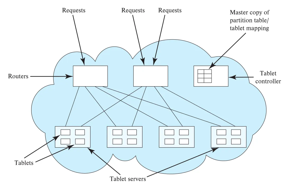 Figure 21.8 · PDF p. 1056 · routers, tablet servers, tablet controller로 구성된 cloud data storage architecture
Figure 21.8은 PNUTS architecture를 느슨하게 기반으로 한 cloud data-storage system 구조를 보여준다. Requests는 routers를 통해 tablet servers로 전달되고, partition table/tablet mapping의 master copy는 tablet controller가 관리한다. Bigtable/HBase는 별도 routers 없이 GFS/HDFS에 저장된 partitioning/tablet-server mapping information을 clients가 읽고 직접 destination을 결정한다.
21.7.2.1 Geographically Distributed Storage
일부 key-value stores는 data를 geographically distributed locations에 replicate한다. 더 나아가 data partitioning도 geography에 걸쳐 수행해, different partitions가 different sets of locations에 replicate되도록 할 수 있다.
Geographic distribution의 첫 번째 목적은 fault tolerance다. 하나의 data center가 fire, earthquake 같은 disaster로 fail해도 service를 계속해야 한다. 지진처럼 한 region의 여러 data centers를 동시에 망가뜨릴 수 있는 failure도 고려한다. 두 번째 목적은 latency 감소다. User와 가까운 region에 copy가 있으면 across-the-world fetch로 인한 hundreds of milliseconds latency를 피할 수 있다.
핵심 trade-off는 remote replication latency와 consistency다.
| 방식 | 장점 | 위험 |
|---|---|---|
| Synchronous geographic replication | Remote location update confirmation을 기다려 stronger durability/consistency를 얻는다. | Cross-region latency 때문에 transaction latency가 커진다. |
| Asynchronous geographic replication | Local update 후 remote confirmation을 기다리지 않고 commit할 수 있다. | Remote replication 전에 failure가 나면 updates를 잃을 수 있다. |
| Application-selectable policy | Application이 request별로 wait/commit policy를 조정할 수 있다. | Correctness 책임 일부가 application design으로 넘어간다. |
21.7.2.2 Index Structure
Key-value store의 각 tablet 안 records는 key로 index된다. Key range queries를 효율적으로 지원하려면 records를 key order로 clustered storage하는 것이 좋다. Mutable storage라면 clustered B+-tree file organization이 좋은 선택이다.
하지만 Bigtable과 HBase는 immutable files를 사용하는 distributed file system 위에 구축된다. Immutable file은 한 번 생성되면 update할 수 없으므로, node split/merge와 pointer updates가 필요한 B+-tree를 그대로 저장하기 어렵다. 그래서 Bigtable/HBase는 Section 14.8.1에서 본 log structured merge tree (LSM tree)의 stepped-merge variant를 사용한다.
LSM tree는 기존 tree를 제자리 update하지 않고, new data 또는 기존 trees merge로 새 tree를 만든다. 따라서 immutable files 위에 잘 맞고, clustered storage와 high insert/update rates를 동시에 지원한다. Apache Cassandra와 MongoDB의 WiredTiger storage structure도 LSM tree 계열을 사용한다.
21.7.3 Support for Transactions
대부분의 key-value stores는 transactions를 제한적으로 지원한다. 보통 single data item에 대한 atomic updates와 serialized updates는 제공한다. 즉, single item operation level에서는 operations가 순차 실행되어 serializability가 자연스럽게 만족된다. 하지만 transaction이 여러 data items를 접근하면, item별 serial execution만으로 transaction-level serializability가 보장되지 않는다.
Megastore와 Spanner 같은 일부 systems는 multiple nodes에 걸친 full ACID transactions를 지원한다. 그러나 대부분의 key-value stores는 multiple data items across nodes에 대한 transactions를 지원하지 않는다.
21.7.3.1 Concurrency Control
Megastore와 Spanner는 locking 기반 concurrency control을 지원한다. Spanner는 timestamp에 기반한 versioning과 database snapshots도 지원하며, 이는 Chapter 23의 multiversion concurrency control과 연결된다.
Bigtable, PNUTS/Sherpa, MongoDB 같은 많은 systems는 single data item에 대한 atomic operations만 지원한다. HBase와 PNUTS는 test-and-set을 제공한다. 이는 data item의 current version이 지정된 version number와 같을 때만 update하는 연산이며, test와 set이 atomically 수행된다. Application은 이를 이용해 Section 23.3.7의 validation-based concurrency control에 가까운 제한적 동시성 제어를 구현할 수 있다.
HBase에는 incrementColumnValue()처럼 column value를 atomically read-and-increment하는 operation이 있고, checkAndPut()처럼 condition을 atomically 검사한 뒤 update하는 operation도 있다. 또한 HBase의 coprocessors는 single data item에서 atomically 실행되는 stored procedures다.
21.7.3.2 Atomic Commit
Bigtable, HBase, PNUTS는 single row에 대한 multiple updates의 atomic commit은 지원하지만, different rows에 걸친 atomic updates는 지원하지 않는다. 이 한계 때문에 이 systems는 secondary indices를 일반적으로 지원하지 않는다. Data item update와 secondary index update를 atomically 묶을 수 없기 때문이다.
PNUTS처럼 일부 system은 deferred updates로 secondary indices 또는 materialized views를 지원한다. Data item update가 발생하면 secondary index/materialized view update message가 messaging service에 추가되고, 해당 update가 적용될 node로 나중에 전달된다. Delivery와 subsequent application은 보장되지만, 적용 전까지 secondary index는 underlying data와 inconsistent할 수 있다. 이는 Chapter 23의 deferred maintenance consistency issue와 연결된다.
반대로 Megastore와 Spanner는 multiple data items, multiple nodes에 걸친 transactions에 대해 two-phase commit (2PC)를 사용해 atomic commit을 보장한다.
21.7.3.3 Dealing with Failures
Tablet server node가 fail하면 같은 tablet copy를 가진 다른 node가 tablet serving을 맡아야 한다. Master node는 node failure를 감지하고 tablet server를 reassign한다. 새 tablet server는 tablet state를 recover해야 하므로, tablet updates는 log에 기록되고 log 자체도 replicated된다.
Bigtable에서는 mapping information과 tablet data가 file system에 저장된다. Tablet data updates는 즉시 flush되지 않을 수 있지만, log data는 flush된다. GFS가 replicated file system data availability를 제공하므로, tablet reassignment 후 새 server는 up-to-date log data에 접근해 recovery를 수행할 수 있다.
Sherpa/PNUTS는 tablets를 cluster의 multiple nodes에 명시적으로 replicate하고, persistent messaging system을 log로 사용한다. Persistent messaging은 log records를 multiple sites에 replicate하여 failure 상황에서도 availability를 보장한다. 새 node가 tablet server가 되기 전, 이전 tablet server가 만든 pending log records를 적용해야 한다.
Replica consistency는 system마다 다르게 처리된다.
| 계열 | 방식 | 의미 |
|---|---|---|
| Bigtable/HBase | GFS/HDFS replication에 의존하고 append를 모든 replicas에 적용한다. | Incomplete appends는 sequence numbers로 감지하고 정리한다. |
| PNUTS | Persistent messaging service로 updates를 all replicas에 delivery한다. | Log delivery 기반 eventual propagation을 사용한다. |
| Megastore/Spanner | Distributed consensus를 사용한다. | Update를 위해 majority of replicas availability가 필요하다. |
| Cassandra/MongoDB | 필요한 replica availability 수를 user/application이 조정할 수 있다. | 낮게 설정하면 conflicting updates가 생기고 later resolution이 필요할 수 있다. |
21.7.4 Managing Without Declarative Queries
Key-value stores는 SQL 같은 query processing facility나 joins 같은 lower-level primitive를 제공하지 않는 경우가 많다. 많은 application은 key로 data를 저장하고 key로 data를 가져오는 access pattern만으로 충분하다. User profile 예시에서는 user identifier가 key가 된다.
하지만 social-networking application처럼 joins가 필요한 경우도 있다. 예를 들어 user에게 friends의 new posts를 보여주는 것은 개념적으로 join이다. Key-value store에서 이를 처리하는 방법은 크게 두 가지다.
| 접근 | 동작 | 비용 |
|---|---|---|
| Application-side join | 먼저 user의 friends set을 찾고, 각 friend object를 query해 recent posts를 모은다. | Query time cost가 크고 many reads가 발생할 수 있다. |
| View materialization | User가 post할 때 각 friend의 data object에 summary를 미리 써 둔다. | Write time cost와 storage cost가 커지지만 read가 빠르다. |
즉, declarative join이 없는 system에서는 read-time computation과 write-time denormalization/materialization 사이에서 trade-off를 선택한다.
21.7.5 Performance Optimizations
Storage system은 physical data location을 client에게 숨긴다. 그러나 자주 join되는 relations를 독립적으로 partition하면 communication cost가 커질 수 있다. 두 relations의 join이 자주 계산된다면, join attributes 기준으로 exactly same way로 partition하는 것이 좋다. 그러면 Section 22.7.4에서 보듯 각 storage site에서 data transfer 없이 parallel join을 수행할 수 있다.
이를 위해 일부 data storage systems는 schema designer가 한 relation의 tuples를 foreign key로 참조하는 다른 relation의 tuples와 같은 partition에 저장하도록 지정할 수 있게 한다. 특정 entity와 관련된 tuples를 같은 partition에 모은 집합을 entity group이라고 한다.
Stored functions/procedures도 data movement를 줄이는 최적화다. HBase 같은 systems는 client가 tuple 또는 entity group에 대해 function을 호출하면, tuples를 client로 가져와 locally execute하는 대신 tuple이 저장된 partition에서 function을 실행한다. Stored tuples가 크고 function result가 작을수록 data transfer 절감 효과가 크다.
또한 많은 systems는 old versions of data items를 일정 기간 후 자동 삭제하거나, 특정 age보다 오래된 data items를 삭제하는 기능을 제공한다. Versioned storage가 무한히 커지는 것을 막는 practical storage management 기능이다.
21.8 Summary
이 장의 흐름은 “data를 어떻게 나눌 것인가”에서 시작해 “나눈 data를 failure와 skew 속에서도 어떻게 안정적으로 제공할 것인가”로 확장된다.
Parallel databases는 data storage와 indexing을 multiple nodes에 분산한다. data partitioning은 relations를 nodes/disks에 나누는 과정이며, round-robin partitioning, hash partitioning, range partitioning이 대표 기법이다. I/O parallelism은 partitioned relation을 여러 disks에서 동시에 읽어 retrieval throughput을 높인다.
Parallelism이 커질수록 skew는 더 심각해진다. Data distribution skew, attribute-value skew, partition skew, execution skew가 서로 다른 원인으로 performance imbalance를 만든다. 이를 줄이기 위해 histograms 기반 balanced range-partitioning vectors, virtual node partitioning, dynamic repartitioning, tablet split/move, consistent hashing이 사용된다.
Failure resilience를 위해 data는 보통 two-way 또는 three-way replication된다. Replicas는 node, rack, data center failure를 고려해 배치되며, master replica와 replica consistency 정책이 필요하다. Updates에 대해 2PC, persistent messaging, consensus protocols, eventual consistency 같은 선택지가 있으며, 선택은 latency, availability, consistency 사이의 trade-off를 결정한다.
Parallel indexing에서는 local index와 global index를 구분해야 한다. Local index는 특정 node의 tuples에 대한 index이고 data와 같은 node에 저장된다. Global index는 multiple nodes의 data를 대상으로 하며, global primary index와 global secondary index로 나뉜다. Global secondary index는 relation의 materialized view처럼 구현될 수 있어 update atomicity 문제가 중요하다.
distributed file system은 many machines에 files를 저장하면서 client에게 single-file-system view를 제공한다. GFS/HDFS는 namenode/datanode 구조, large blocks, replicated blocks, write-once-read-many model로 huge files를 안정적으로 저장한다. 그러나 small records의 frequent update workload에는 key-value store가 더 적합하다.
parallel key-value store는 billions of small records를 key 기반으로 저장하고 검색하도록 설계되었다. Flexible schema, wide-column stores, document stores, JSON representation, column family, tablet/tablet server/master/router architecture, geographic replication, LSM tree, limited transactions, materialized view style denormalization이 핵심 설계 요소다.
연결 관계
- Chapter 8: JSON, semi-structured data, complex data types 논의가 document store와 data representation으로 이어진다.
- Chapter 12-14: physical storage, file organization, B+ tree, LSM tree가 tablet 내부 index structure 선택의 기반이다.
- Chapter 16: query optimization에서의 cost와 data movement 개념이 co-partitioning과 entity group 설계로 이어진다.
- Chapter 17-19: transactions, concurrency control, recovery가 key-value stores의 limited transaction, test-and-set, logging, atomic commit 문제로 확장된다.
- Chapter 20: data-center topology와 rack/data-center failure model이 replica placement와 geographic replication을 설명하는 배경이 된다.
- Chapter 22-23: parallel query processing, distributed concurrency control, distributed recovery, distributed consensus가 이 장의 storage architecture 위에서 동작한다.
오해하기 쉬운 내용
Distributed file system과parallel key-value store는 모두 distributed storage지만 abstraction이 다르다. 전자는 file/block abstraction, 후자는 key/value 또는 row/column abstraction이다.Replication은 capacity 증가가 아니라 availability/fault tolerance를 위한 설계다. Read throughput 향상에도 도움이 될 수 있지만 consistency 비용을 만든다.Hash partitioning은 균등 분산에 유리하지만 range query locality가 약하다.Range partitioning은 range query에 유리하지만 skew 관리가 필요하다.Local index는 node-local data만 찾는다. 전체 relation을 대상으로 특정 secondary attribute를 찾으려면global secondary index가 필요하다.- Key-value store의 single-item atomicity는 transaction-level serializability와 다르다. 여러 keys/rows를 함께 update하면 별도 atomic commit이 필요하다.
- Eventual consistency는 “항상 틀려도 된다”가 아니라, delayed propagation 동안 stale/inconsistent read가 가능하다는 뜻이다.
면접 질문
round-robin partitioning,hash partitioning,range partitioning을 scan, point query, range query 기준으로 비교하라.data distribution skew,attribute-value skew,partition skew,execution skew가 어떻게 다른지 설명하라.virtual node partitioning이 elasticity와 skew mitigation에 왜 도움이 되는가?- Tablet split/move 이후 router의 partition table이 stale할 때 request는 어떻게 처리되는가?
local index,global primary index,global secondary index의 차이를 설명하라.- HDFS가
write-once-read-many access model을 택한 이유를 replica consistency 관점에서 설명하라. - Key-value store에서 secondary index 유지가 어려운 이유를 atomic commit 관점에서 설명하라.
- Geographic replication에서 synchronous replication과 asynchronous replication의 latency/consistency trade-off를 비교하라.
LSM tree가 immutable distributed file system 위의 key-value store에 잘 맞는 이유는 무엇인가?- SQL join이 없는 key-value store에서 social feed를 구현할 때 application-side join과 materialized view 방식의 trade-off는 무엇인가?
용어 회수
data storage system, I/O parallelism, data partitioning, horizontal partitioning, vertical partitioning, round-robin partitioning, hash partitioning, range partitioning, partitioning vector, point query, range query, skew, data distribution skew, attribute-value skew, partition skew, execution skew, balanced range-partitioning vector, histogram, virtual node, elasticity, tablet, partition table, master node, router, consistent hashing, distributed hash table, DHT, replication, replica, master replica, eventual consistency, two-phase commit, 2PC, persistent messaging, consensus protocols, local index, global index, global primary index, global secondary index, materialized view, distributed file system, GFS, HDFS, namenode, datanode, BackupNode, block ID, write-once-read-many access model, parallel key-value store, key-value store, put(table, key, value), get(table, key), wide-column store, document store, JSON, column family, tablet server, tablet controller, geographically distributed storage, LSM tree, test-and-set, checkAndPut(), incrementColumnValue(), coprocessor, entity group.