개요
이 장은 parallel database system에서 read-only query를 여러 nodes에 나누어 처리하는 방법을 다룬다. 초점은 decision support systems처럼 very large data를 대상으로 long-running queries를 acceptable response time 안에 끝내야 하는 상황이다. Transaction processing처럼 많은 short update queries를 처리하는 문제는 Chapter 23의 parallel/distributed transaction processing에서 다룬다.
핵심 질문은 두 가지다. 첫째, single query 안의 operation을 어떻게 여러 nodes에서 나눠 실행할 것인가. 둘째, query plan 전체를 어떻게 parallel execution plan으로 바꾸어 network transfer, skew, startup cost, fault tolerance를 함께 관리할 것인가. 앞부분은 relational query processing에 집중하고, 뒤에서는 streaming data와 multiple data sources를 대상으로 한 distributed query processing까지 확장한다.
핵심 개념
interquery parallelism은 여러 queries를 서로 병렬로 실행해 throughput을 높이는 방식이다.intraquery parallelism은 하나의 query 내부를 병렬화해 long-running query의 response time을 줄이는 방식이다.intraoperation parallelism은 sort, join, aggregate 같은 하나의 operator를 여러 nodes에서 나누어 실행하는 것이다.interoperation parallelism은 query operator tree의 서로 다른 operators를 동시에 실행하는 것이다. 여기에는pipelined parallelism과independent parallelism이 포함된다.- 이 장의 기본 설명 모델은 shared-nothing architecture의 nodes
N1, N2, ..., Nn이다. Shared-memory/shared-disk system도 data transfer를 memory/disk 공유로 시뮬레이션할 수 있으므로 같은 알고리즘 틀을 적용할 수 있다. - Parallel query processing은 항상 data transfer, load balance, skew, memory pressure, network cost, fault tolerance 사이의 trade-off를 가진다.
세부 정리
22.1 Overview
Parallelism은 database system에서 두 층위로 사용된다. interquery parallelism은 여러 independent queries를 동시에 실행한다. 이는 transaction processing system에서 transactions per second를 늘리는 데 중요하지만, individual transaction의 response time을 줄이지는 않는다. 반면 intraquery parallelism은 하나의 query를 쪼개 실행하므로 long-running analytical query의 latency를 줄이는 데 핵심이다.
Single query의 execution은 selections, joins, aggregate operations, sort 같은 여러 operations로 이루어진다. Large-scale parallelism의 핵심은 각 operation 자체를 parallelize하는 것이다. Relation의 tuple 수는 매우 클 수 있으므로, 같은 operation을 여러 data partitions에 동시에 적용하는 intraoperation parallelism은 database에서 자연스럽다.
예를 들어 relation이 sort attribute로 range partitioning되어 있다면 각 partition을 병렬로 local sort한 뒤 결과를 concatenate하면 전체 sorted relation을 얻을 수 있다. 이처럼 query를 parallelize하는 가장 직접적인 방법은 individual operations를 parallelize하는 것이다.
또 다른 parallelism source는 query의 operator tree다. 서로 dependency가 없는 operations는 동시에 평가할 수 있고, 한 operation의 output을 다른 operation으로 바로 넘기는 pipeline도 가능하다. 이런 형태는 interoperation parallelism이다.
| 구분 | 목표 | 대표 예 | 한계 |
|---|---|---|---|
interquery parallelism | 동시에 많은 queries 처리 | 많은 OLTP transactions 병렬 실행 | 개별 query/transaction latency는 그대로일 수 있다. |
intraoperation parallelism | single operator를 여러 data partitions에서 병렬 실행 | parallel sort, parallel join, parallel aggregate | data redistribution과 skew 관리가 필요하다. |
interoperation parallelism | query plan의 여러 operators를 동시에 실행 | pipeline, independent subplans | operator 수가 tuple 수보다 훨씬 적어 scale-out 한계가 있다. |
두 방식은 상호 배타적이지 않다. Query 하나 안에서 intraoperation parallelism과 interoperation parallelism을 동시에 사용할 수 있다. 다만 typical query는 operators 수보다 각 operator가 처리하는 tuples 수가 훨씬 많으므로, parallelism 증가에 따라 더 잘 scale하는 것은 보통 intraoperation parallelism이다. Interoperation parallelism은 특히 multi-core shared-memory systems에서 중요하다.
이 장은 설명을 단순화하기 위해 shared-nothing architecture를 가정한다. 각 node는 하나 이상의 disks를 가질 수 있지만, node 내부 disk partitioning은 RAID 같은 storage-level parallelism으로 처리한다고 본다. Shared-memory architecture에서는 node 간 data transfer가 shared memory access로, shared-disk architecture에서는 shared disk access로 대체될 수 있다. 현대 parallel systems는 multi-core shared-memory machines를 여러 대 shared-nothing 방식으로 묶은 hybrid architecture가 많고, 이때 각 core를 논리적 node로 생각할 수 있다.
22.2 Parallel Sort
Relation r이 sort attributes로 이미 range-partitioned되어 있다면, 각 node가 자기 partition을 local sort하고 partition 순서대로 concatenate하면 된다. 전체 relation read time은 parallel disk access 덕분에 대략 nodes 수 n에 비례해 줄어든다.
Relation이 다른 방식으로 partitioned되어 있거나 sort attribute와 partitioning attribute가 다르면 두 가지 대표 방법을 쓴다.
range-partitioning sort: sort attributes 기준으로 relation을 다시 range partitioning한 뒤 각 partition을 local sort한다.parallel external sort-merge: 각 node가 local data를 먼저 sort하고, sorted runs를 range partitioning하며 병합한다.
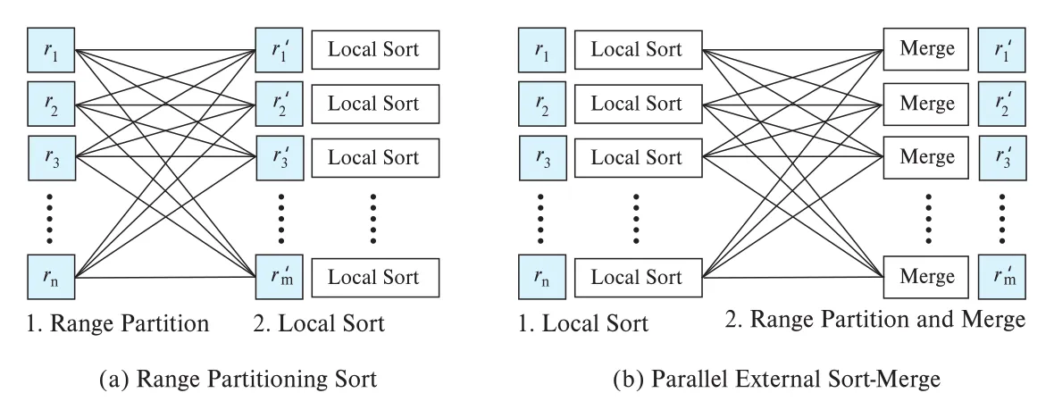 Figure 22.1 · PDF p. 1071 · range-partitioning sort와 parallel external sort-merge의 처리 흐름
Figure 22.1(a)의 range-partitioning sort는 두 단계다. 먼저 모든 nodes가 자기 disk에서 tuples를 읽고, sort attribute의 range partition function에 따라 destination node로 tuples를 보낸다. Destination node는 자기 range에 속한 tuples를 받아 local disk에 임시 저장한다. 이 단계는 disk I/O와 network communication을 모두 사용한다. 그 다음 각 node가 자기 partition을 independently local sort한다. 첫 단계의 range partitioning이 i < j인 node Ni의 key values가 Nj보다 작도록 보장하므로, 마지막 merge는 사실상 concatenate에 가깝다.
이 방법에서 가장 중요한 조건은 balanced range-partitioning vector다. Partition vector가 skewed하면 어떤 node는 너무 많은 tuples를 받아 local sort와 network receive에서 bottleneck이 된다. Chapter 21의 histogram 기반 balanced range-partitioning vector와 virtual node partitioning은 이 skew를 줄이기 위한 기반이다.
Figure 22.1(b)의 parallel external sort-merge는 relation이 이미 어떤 방식으로든 nodes에 partitioned되어 있을 때 사용할 수 있다. 각 node Ni가 자기 local data를 sort하고, 이후 sorted runs를 같은 partition vector로 여러 destination nodes에 range-partition하면서 merge한다. 각 destination node는 여러 source nodes에서 sorted streams를 받아 single sorted run으로 merge한다. 마지막에는 destination nodes의 sorted runs를 concatenate한다.
Parallel external sort-merge에는 흥미로운 execution skew 위험이 있다. 모든 source nodes가 먼저 partition 1의 tuples만 N1으로 보내고, 그 다음 partition 2만 N2로 보내면, send는 병렬이어도 receive는 사실상 N1, N2, … 순서로 순차화된다. 이를 피하려면 source node i에서 destination node j로 가는 sorted sequence Si,j를 multiple blocks로 쪼갠다. 각 source node는 모든 destinations에 첫 번째 block을 보내고, 그 다음 두 번째 block을 보내는 식으로 진행한다. 이렇게 하면 모든 destination nodes가 동시에 receive/merge할 수 있다. Tuples는 network overhead를 줄이기 위해 individual tuple이 아니라 blocks 단위로 전송한다.
정리하면 parallel sort의 선택은 현재 partitioning, sort attribute, network cost, skew 가능성에 달려 있다. 이미 sort attribute로 range partitioned되어 있으면 local sort가 가장 단순하고, 그렇지 않으면 redistribution cost를 감수하면서 range partitioning 또는 parallel external sort-merge를 사용한다.
22.3 Parallel Join
Parallel join algorithms는 input relations의 tuples를 여러 nodes에 나누고, 각 node가 join 결과의 일부를 locally compute하게 만든다. 핵심은 “어떤 tuple 쌍이 서로 join될 가능성이 있는가”를 기준으로 data를 배치하는 것이다. Equi-join처럼 join key가 명확하면 같은 key range/hash bucket을 같은 node에 보내면 되고, inequality join처럼 tuple pair 조합이 넓게 열려 있으면 replication이 필요해진다.
22.3.1 Partitioned Join
partitioned join은 equi-join 조건, 예를 들어 r ⋈r.A=s.B s에 사용할 수 있다. 두 relations r, s를 join attributes 기준으로 같은 partitioning function에 따라 m개 partitions로 나눈다. Range partitioning이면 같은 partition vector를, hash partitioning이면 같은 hash function을 써야 한다. 그러면 같은 join key를 가진 r tuple과 s tuple이 같은 node로 가므로 각 node는 local join만 수행하면 된다.
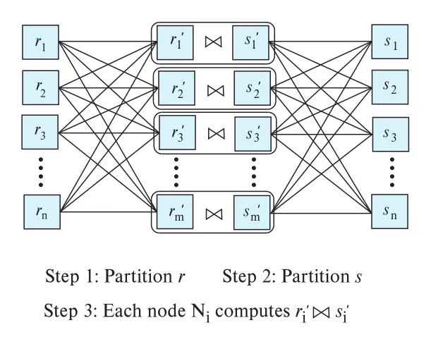 Figure 22.2 · PDF p. 1073 · 두 relations를 같은 join key partitioning으로 재분배한 뒤 node별 local join을 수행하는 partitioned parallel join
Figure 22.2의 흐름은 세 단계다.
| 단계 | 동작 |
|---|---|
| 1 | 각 node가 relation r의 local tuples를 scan하고 join attribute value로 destination partition rj를 계산해 node Nj로 보낸다. |
| 2 | 같은 방식으로 relation s를 partition sj로 보낸다. 각 destination node는 동시에 receive thread로 tuples를 받아 local disk에 저장할 수 있다. |
| 3 | 각 node Ni가 local partitions ri와 si를 원하는 join algorithm으로 join한다. |
Partitioned join은 inner equi-join뿐 아니라 left/right/full outer join에도 사용할 수 있다. Partitioning이 join attributes 기준으로 되어 있으면 matching 가능성이 있는 tuples가 같은 node에 오므로, 각 node가 local outer join을 계산해도 전체 outer join 의미가 유지된다. Natural join도 equijoin 후 projection으로 볼 수 있으므로 partitioned join으로 처리할 수 있다.
이미 r 또는 s가 join attributes 기준으로 partitioned되어 있으면 repartition work가 줄어든다. 두 relation이 둘 다 같은 방식으로 partitioned되어 있으면 data transfer 없이 local join에 가깝게 처리할 수 있다. 반대로 partitioning attributes가 join attributes와 다르면 redistribution이 필요하다.
Local join algorithm에 따라 세부 최적화가 달라진다.
| Local join | Parallel 형태 | 핵심 최적화 |
|---|---|---|
| Hash join | partitioned parallel hash join | Node 간 partitioning hash h0()와 local hash join partitioning hash h1()를 다르게 써야 한다. Incoming tuples를 받는 즉시 local hash partitions로 나누면 disk write/read를 줄인다. |
| Hybrid hash join | partitioned parallel hash join의 변형 | Build relation의 일부 partition s0를 memory에 유지하고, probe relation의 대응 partition r0가 도착하면 바로 in-memory index를 probe한다. |
| Merge join | partitioned parallel merge join | Received partitions ri, si를 local sort 후 merge한다. Incoming tuples를 곧바로 run generation에 넣어 불필요한 disk round-trip을 줄일 수 있다. |
| Nested-loops join | partitioned parallel nested-loop join 또는 partitioned parallel indexed nested-loops join | 각 node가 자기 ri, si에 대해 nested-loop/indexed nested-loop join을 수행한다. |
22.3.2 Fragment-and-Replicate Join
fragment-and-replicate join은 partitioning만으로 join pair를 localize하기 어려운 join에 사용한다. 예를 들어 inequality join r ⋈r.a<s.b s에서는 r의 어떤 tuple이 s의 광범위한 tuples와 join될 수 있으므로, ri와 si만 비교하는 partitioned join으로는 충분하지 않다.
특수한 형태인 asymmetric fragment-and-replicate join, 또는 broadcast join은 다음처럼 동작한다.
- 한 relation, 예를 들어
r을 여러 nodes에 partition한다. 이미 partitioned되어 있으면 그대로 쓴다. - 다른 relation
s를 모든 nodes에 replicate한다. - 각 node
Ni가ri와 전체s를 locally join한다.
Broadcast join은 inequality join뿐 아니라 equi-join에서도 유용하다. 특히 s가 small relation이고 r이 large relation이면, large relation을 repartition하는 것보다 small relation을 모든 nodes에 broadcast하는 편이 싸다.
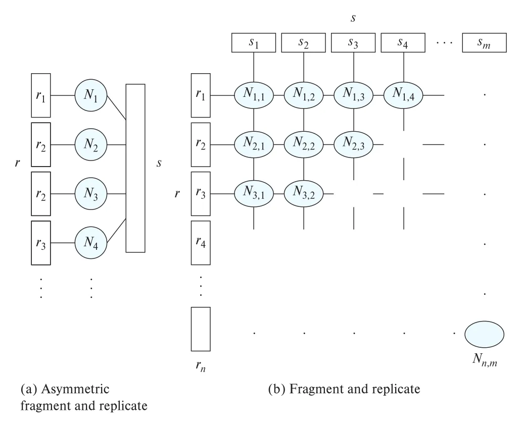 Figure 22.3 · PDF p. 1076 · asymmetric broadcast join과 symmetric fragment-and-replicate join의 data 배치
일반형인 symmetric fragment-and-replicate join은 r을 n partitions, s를 m partitions로 나누고, 최소 m * n nodes를 사용한다. Node Ni,j는 ri와 sj의 join을 계산한다. 이를 위해 ri는 row 방향 nodes Ni,1 ... Ni,m에 replicate되고, sj는 column 방향 nodes N1,j ... Nn,j에 replicate된다. 이 방식은 모든 tuple pair를 검사할 수 있으므로 join condition 제한이 거의 없다.
비용은 replication이다. r의 각 tuple은 m번, s의 각 tuple은 n번 복제된다. 따라서 symmetric fragment-and-replicate는 equi-join처럼 partitioned join이 가능한 경우에는 보통 비싸고, non-equi join처럼 partitioning으로 해결되지 않을 때 사용한다.
Outer join에는 주의가 필요하다. r ⟕θ s에서 s를 replicate하고 r을 partition하면 각 node가 자기 ri와 전체 s를 보므로 left outer join을 locally 계산할 수 있다. 하지만 s가 fragmented되고 r이 replicated되면 어떤 r tuple이 현재 node의 si에는 match가 없어도 다른 partition sj에는 match가 있을 수 있다. 이 경우 null-extended output을 locally 결정할 수 없으므로 left outer join 의미가 깨진다. 같은 이유로 full outer join과 symmetric fragment-and-replicate의 조합도 조심해야 한다.
22.3.3 Handling Skew in Parallel Joins
Parallel join에서 skew는 전체 completion time을 지배한다. 대부분 nodes가 일을 끝내고 idle 상태가 되어도, 한 node가 heavy join partition을 붙잡고 있으면 query는 끝나지 않는다. Storage partitioning에서는 tuple 수 균형이 중요했지만, join에서는 node별 join execution time 균형이 더 중요하다.
Hash partitioning은 good hash function을 쓰면 보통 load balance가 좋다. 그러나 join attribute의 특정 값이 매우 자주 등장하면 같은 hash bucket으로 몰려 skew가 생긴다. Range partitioning은 range boundary를 조심해서 고르지 않으면 더 쉽게 join skew가 생긴다. Cost estimation에는 join attributes의 histograms가 필요하며, heuristic하게 각 node Ni의 join cost를 |ri| + |si|에 비례한다고 보고 range partition vector를 고를 수 있다.
Skew 완화에는 두 접근이 있다.
| 접근 | 설명 |
|---|---|
join skew avoidance | Balanced partitioning, virtual-node partitioning처럼 실행 전에 skew를 줄이도록 partitioning한다. Virtual nodes를 real nodes에 round-robin으로 배치하면 skewed virtual nodes가 여러 real nodes에 퍼진다. |
| Dynamic handling | 실행 중 progress를 감시하다가 idle real node가 busy real node의 unprocessed virtual node work를 가져와 처리한다. |
Dynamic handling은 work stealing의 한 형태다. 각 real node는 virtual node 하나씩 join task를 처리한다. 어떤 node가 자기 tasks를 모두 끝냈는데 다른 node에는 아직 여러 virtual nodes가 남아 있으면, idle node가 그 중 하나의 data copy를 가져와 join을 수행한다. Shared-memory system에서는 모든 data에 빠르게 접근할 수 있어 work stealing 비용이 작다. Shared-nothing system에서는 data movement가 필요할 수 있지만, heavy skew로 전체 query가 지연되는 것보다 data movement overhead를 감수하는 편이 낫다.
22.4 Other Operations
22.4.1 Other Relational Operations
Join 외의 relational operations도 같은 원리로 parallelize할 수 있다.
| Operation | Parallelization 방식 | 주의점 |
|---|---|---|
Selection σθ(r) | Predicate가 partitioning attribute의 equality이면 single node에서 처리한다. Range predicate이고 relation이 해당 attribute로 range-partitioned되어 있으면 overlapping partitions만 처리한다. 그 외에는 모든 nodes에서 parallel selection한다. | Partitioning attribute와 predicate attribute가 맞으면 불필요한 node access를 줄인다. |
| Duplicate elimination | Parallel sort를 쓰면서 duplicate가 나타나는 즉시 제거하거나, tuples를 hash/range partitioning한 뒤 node별 local duplicate elimination을 수행한다. | 같은 duplicate candidates가 같은 node로 가야 한다. |
| Projection | Duplicate elimination이 없으면 disk에서 tuples를 읽으며 parallel projection하면 된다. Duplicates 제거가 필요하면 duplicate elimination 기법을 결합한다. | SQL projection의 duplicate semantics에 주의한다. |
| Aggregation | Grouping attributes로 relation을 partition하고 각 node가 local aggregate를 계산한다. 이미 grouping attributes로 partitioned되어 있으면 repartition step을 생략한다. | Group-by key skew가 있으면 특정 node에 groups가 몰릴 수 있다. |
Aggregation은 partial aggregation이 특히 중요하다. 예를 들어 A로 group by하고 sum(B)를 계산한다면, 각 node가 먼저 자기 local tuples에 대해 A별 partial sum을 만든다. 그 다음 partial sums만 grouping attribute A로 repartition하고, destination nodes에서 partial sums를 다시 aggregate한다. 이 방식은 raw tuples 대신 compact partial results를 network로 보내므로 transfer cost가 줄어든다. min, max에도 쉽게 적용되고, count, avg는 count/sum 같은 보조 값을 함께 보내는 식으로 확장할 수 있다.
Aggregation skew는 join skew보다 다루기 쉬운 편이다. Aggregation cost는 보통 input size에 비례하므로 good hash function으로 group-by values를 균등 분산하면 충분한 경우가 많다. 다만 특정 group-by values가 매우 자주 등장하면 hashing만으로 불균형이 생긴다. Partial aggregation은 이런 상황에서 매우 효과적이다. Partial aggregation이 불가능하면, overloaded node의 아직 처리되지 않은 key values나 virtual nodes를 다른 real nodes에 reassign하는 dynamic handling이 필요하다.
22.4.2 Map and Reduce Operations
MapReduce는 parallel data processing programs를 쉽게 작성하도록 만든 paradigm이다. Programmer가 제공한 map() function은 input record 하나를 받아 zero or more output records를 낸다. 각 output record는 (key, value) 형태이며, 여기서 key는 intermediate key 또는 reduce key 역할을 한다. System은 같은 intermediate key를 가진 records를 모아 programmer가 제공한 reduce() function을 호출한다.
Relational 관점에서 map()은 project operation의 일반화다. Projection은 input record 하나에서 output record 하나를 만들지만, map은 0개, 1개, 또는 여러 output records를 만들 수 있다. reduce()는 grouped values를 받아 결과를 만들므로 user-defined aggregation function으로 볼 수 있다.
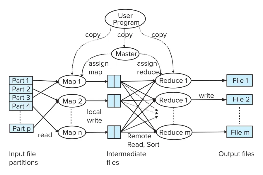 Figure 22.4 · PDF p. 1080 · input partitions, map tasks, intermediate files, reduce tasks, output files로 이어지는 MapReduce job 병렬 처리
Figure 22.4의 MapReduce execution은 database의 virtual-node partitioning과 매우 닮았다.
| 구성 | 이 장의 용어와 연결 | 역할 |
|---|---|---|
| Input file partitions | virtual nodes | 여러 tasks로 나뉘어 map workers가 처리한다. |
| Workers | real nodes 또는 cores | map/reduce functions를 실행하는 processes다. 보통 machine의 processor cores 수와 맞춘다. |
| Scheduler/master | task assignment controller | worker가 task를 끝내면 새 task를 배정한다. |
| Intermediate files | repartitioned map output | reduce key 기준으로 range/hash partitioning된다. |
| Reduce tasks | reduce-key partitions | 같은 reduce key를 가진 records를 모아 reduce function을 호출한다. |
Map과 reduce 사이의 핵심 단계는 repartitioning이다. Map output records는 reduce key 기준으로 range partitioning 또는 hash partitioning되어, 같은 key를 가진 records가 같은 reduce task로 간다. 이는 relational aggregation을 group-by key로 repartition하는 것과 동일한 구조다.
Reduce task 내부에서는 records가 reduce key로 sorted 또는 grouped되어 같은 key의 values가 함께 모인다. Reduce task 하나가 여러 reduce key values를 포함할 수 있지만, reduce() function 호출 하나는 single reduce key에 대한 values collection을 처리한다.
MapReduce에서 tasks는 real nodes보다 훨씬 많다. 이는 Chapter 21의 virtual node partitioning과 같아서 skew를 줄인다. Workers가 task를 끝낼 때마다 scheduler가 다음 task를 주기 때문에, 느린 task 일부가 전체 job을 붙잡는 문제를 완화할 수 있다. 또한 partial aggregation에 해당하는 combiner는 map side에서 먼저 aggregate하여 network shuffle 비용과 skew를 줄인다.
MapReduce implementations는 execution 중 node failure가 나도 processing을 계속할 수 있는 fault tolerance 기법을 포함한다. 이는 이후 Section 22.5.4의 query plan fault tolerance와 연결된다.
22.5 Parallel Evaluation of Query Plans
앞 절까지는 하나의 operation을 parallelize하는 intraoperation parallelism을 보았다. 이제 query가 여러 operations를 포함할 때 전체 execution plan을 어떻게 병렬 평가하는지가 문제다. 핵심 모델은 exchange operator model이다. 이 모델은 parallel query processing을 두 종류의 단계로 나눈다.
exchange operator가 data를 필요한 방식으로 partition/repartition/broadcast/collect한다.- Exchange 사이의 operators는 local data만 사용해 centralized DBMS의 operator처럼 실행된다.
이 분리는 강력하다. Parallelism을 모르는 기존 local query engine을 거의 그대로 사용하면서, data movement만 exchange operator로 캡슐화할 수 있기 때문이다.
22.5.1 Interoperation Parallelism
interoperation parallelism은 한 query 안의 여러 operators를 동시에 실행하는 방식이다. 두 형태가 있다.
| 형태 | 의미 | 장점 | 한계 |
|---|---|---|---|
pipelined parallelism | Operator A가 output tuples를 생성하는 동시에 operator B가 이를 소비한다. | Intermediate results를 disk에 쓰지 않아도 되고 A/B가 동시에 실행된다. | Pipeline length가 짧고 blocking operators에서는 사용할 수 없다. |
independent parallelism | 서로 dependency가 없는 subexpressions를 동시에 실행한다. | Query tree의 독립 branches를 동시에 처리한다. | 독립 branch 수가 많지 않아 high degree parallelism에는 한계가 있다. |
22.5.1.1 Pipelined Parallelism
Pipelining은 sequential query processing에서도 intermediate results를 disk에 쓰지 않기 위해 사용된다. Parallel system에서는 여기에 추가로 producer operator와 consumer operator를 다른 nodes 또는 cores에서 동시에 실행할 수 있다는 장점이 생긴다. 예를 들어 operator A가 tuples를 생성하는 동안 operator B가 이미 그 tuples를 소비하면, A와 B가 겹쳐 실행된다.
하지만 pipelined parallelism은 scale-out 효과가 제한적이다. 첫째, query plan의 pipeline chain은 보통 충분히 길지 않다. 둘째, set-difference 같은 blocking operator는 input을 모두 읽기 전 output을 만들지 않으므로 pipeline에 맞지 않는다. 셋째, 어떤 operator 하나의 cost가 압도적으로 크면 다른 operators를 병렬로 실행해도 speedup은 작다. 그래서 높은 degree of parallelism에서는 partitioning 기반 intraoperation parallelism이 더 중요하다.
Centralized DBMS에서는 pull model 또는 demand-driven iterator model이 널리 쓰인다. Consumer가 “다음 tuple”을 요청하면 producer가 tuple을 만들어 준다. 하지만 parallel DBMS에서는 push model이 선호된다. Producer가 tuples를 생성해 consumer로 밀어 넣어야 producer와 consumer가 동시에 실행될 수 있기 때문이다.
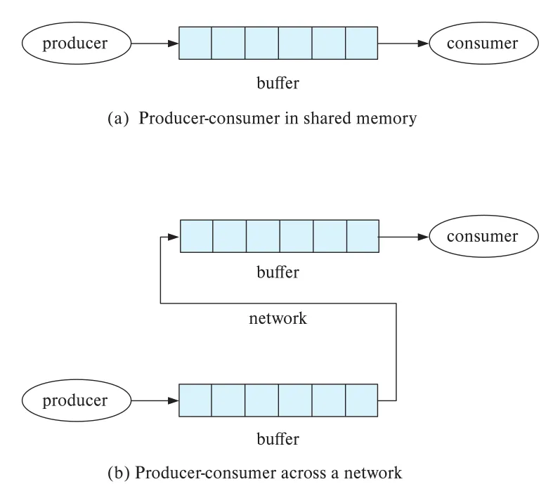 Figure 22.5 · PDF p. 1083 · shared memory 또는 network를 사이에 둔 producer-consumer buffer 구조
Figure 22.5는 push model에 필요한 buffer를 보여준다. Producer와 consumer가 같은 node에 있으면 shared memory buffer를 사용할 수 있다. 다른 nodes에 있으면 producer side buffer와 consumer side buffer가 필요하고, tuples는 network를 통해 전송된다. Network에서는 message당 overhead가 크므로 tuples를 하나씩 보내지 않고 batch로 모아 보낸다. Shared memory buffer에서도 mutual exclusion overhead를 줄이기 위해 tuple 단위보다 batch 단위 insert/retrieve가 유리하다.
Pull model은 producer와 consumer 중 한쪽만 실행되므로 buffer contention은 줄지만 concurrency를 잃는다. Push model은 buffer coordination 비용을 내는 대신 producer-consumer parallelism을 얻는다.
22.5.1.2 Independent Parallelism
independent parallelism은 query expression에서 서로 의존하지 않는 operations를 동시에 실행한다. 예를 들어 r1 ⋈ r2 ⋈ r3 ⋈ r4에서 먼저 t1 <- r1 ⋈ r2와 t2 <- r3 ⋈ r4를 동시에 계산할 수 있다. 두 join은 서로 input/output dependency가 없기 때문이다. 이후 t1 ⋈ t2는 두 intermediate results가 모두 있어야 하므로 independent parallelism으로 동시에 시작할 수 없다.
Independent parallelism은 낮은 degree of parallelism에서는 유용하지만, high parallel system에서는 제공할 수 있는 parallel tasks 수가 작아 한계가 있다.
22.5.2 The Exchange Operator Model
exchange-operator model은 Volcano parallel database가 널리 알린 parallelization model이다. Exchange operation은 data interchange를 담당하고, 나머지 operators는 local data만 처리한다. 즉, parallel plan은 “exchange로 data 위치를 맞추고, local operators로 계산한다”는 반복 구조로 표현된다.
Exchange operator는 두 구성요소를 가진다.
| 구성요소 | 위치 | 역할 |
|---|---|---|
| Partition scheme | source nodes | outgoing data를 hash/range/broadcast/collect 방식으로 destination에 나눈다. |
| Merge scheme | destination nodes | multiple source nodes에서 온 incoming data를 합친다. random merge 또는 ordered merge가 가능하다. |
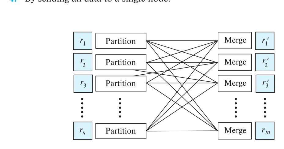 Figure 22.6 · PDF p. 1084 · source nodes의 Partition과 destination nodes의 Merge로 구성된 exchange operator
Exchange operator가 지원하는 data movement는 다음과 같다.
| 방식 | 사용 맥락 |
|---|---|
| Hash partitioning | Join/aggregation key 기준으로 같은 key를 같은 node에 모은다. |
| Range partitioning | Sort/range query/ordered merge가 필요한 경우에 사용한다. |
| Broadcasting | Small relation을 모든 nodes에 보내 asymmetric fragment-and-replicate join을 수행한다. |
| Collect to single node | 최종 결과를 single site에 모으는 마지막 단계에 사용한다. |
Destination의 merge는 두 방식으로 나뉜다. random merge는 source tuples를 도착 순서대로 저장한다. Network delay와 machine speed 때문에 결과 order는 nondeterministic할 수 있다. ordered merge는 각 source input이 sorted일 때 sort order를 활용해 sorted local output을 만든다. Parallel external sort-merge는 local sort 후 exchange의 range partitioning과 ordered merge를 결합한 예다.
앞서 본 parallel operators는 모두 exchange와 local operator의 sequence로 모델링할 수 있다.
| Parallel operation | Exchange model 표현 |
|---|---|
| Range partitioning sort | range partitioning exchange + destination local sort |
| Parallel external sort-merge | source local sort + range partitioning exchange + ordered merge |
| Partitioned join | join attributes 기준 exchange + destination local join |
| Asymmetric fragment-and-replicate join | small relation broadcast exchange + local join |
| Symmetric fragment-and-replicate join | partition + partial broadcast exchange + local join |
| Aggregation | grouping attributes 기준 hash partitioning exchange + local aggregation |
| Partial aggregation | exchange 전에 source local aggregation을 추가 |
Exchange model의 큰 장점은 local operators가 parallelism을 몰라도 된다는 점이다. Local hash join, local sort, local aggregation은 centralized DBMS에서처럼 동작하고, data movement만 exchange가 담당한다. 그래서 기존 query engine code를 크게 바꾸지 않고 parallel DBMS를 구현할 수 있다.
다만 모든 operator가 parallelism을 몰라도 되는 것은 아니다. Parallel data-store의 indexed nested-loop join은 inner index lookup마다 remote access가 필요할 수 있으므로 underlying parallel storage를 알아야 한다. Shared-memory system에서는 여러 processors가 shared hash table이나 shared index를 접근하는 구현도 가능하다.
Exchange operator는 parallel pipeline에서 push model을 구현하면서 local operators에는 pull model을 유지하게 해 준다. Source side exchange는 local operator에서 demand-driven 방식으로 tuples를 여러 개 pull해 destination별 batch를 만들고, batch를 network로 보낸다. Destination side exchange는 받은 tuples를 buffer에 merge해 두고, local consumer operator는 이를 pull model로 소비한다.
22.5.3 Putting It All Together
Figure 22.7은 query r.C,s.D γsum(s.E) (r ⋈r.A=s.B s)를 sequential plan과 parallel plans로 보여준다. 이 query는 먼저 r.A = s.B join을 수행하고, join result를 (r.C, s.D)로 group by하여 sum(s.E)를 계산한다.
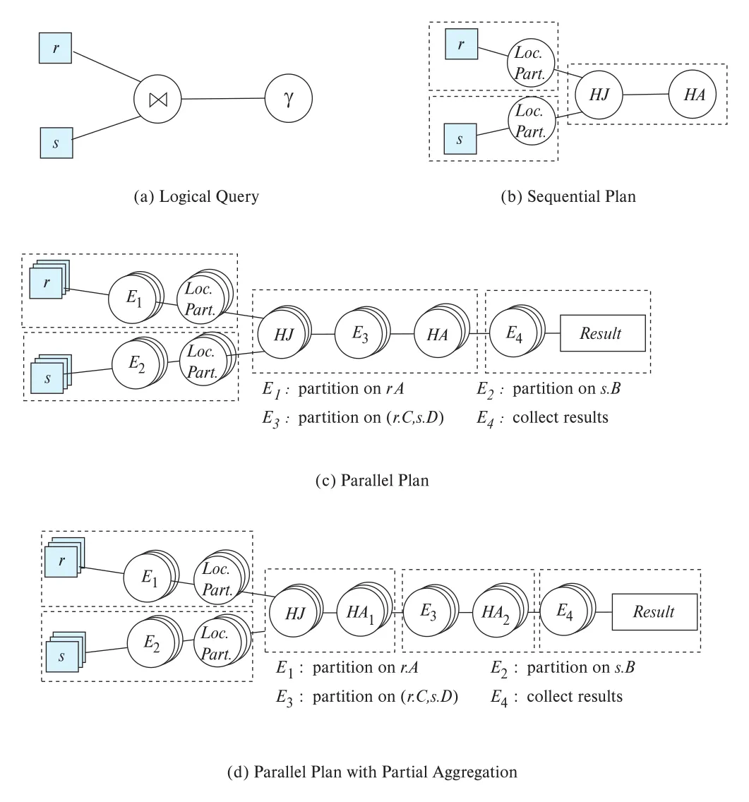 Figure 22.7 · PDF p. 1087 · hash join과 hash aggregation을 exchange operators로 병렬화한 query execution plans
Sequential plan은 HJ hash join과 HA hash aggregation으로 구성된다. Hash join은 local partitioning stages로 r과 s를 각각 join attributes 기준 partition하고, 대응 partitions를 join한다. Join output은 hash aggregation으로 pipeline된다.
Parallel plan에서는 r과 s가 이미 여러 nodes에 partitioned되어 있지만 join attributes 기준은 아니라고 가정한다. 그래서 E1 exchange가 r.A로 r을 repartition하고, E2 exchange가 s.B로 s를 repartition한다. 각 node는 local hash join을 수행한다. Local hash join 내부에서도 partitions가 memory에 fit하지 않으면 local partitioning step이 필요하며, Figure 22.7의 Loc. Part.가 이를 나타낸다.
Join output은 grouping attributes (r.C, s.D) 기준으로 E3 exchange를 거쳐 repartition된다. Destination nodes에서는 hash aggregation HA가 local aggregate를 계산한다. 마지막 E4 exchange는 final aggregate results를 central location으로 collect한다.
Figure 22.7(d)는 partial aggregation을 추가한 plan이다. Local hash join 뒤 HA1이 먼저 local partial aggregation을 수행하고, 그 결과만 E3로 repartition한다. Destination nodes의 HA2가 final aggregate values를 계산한다. Partial aggregation은 network transfer를 줄이지만, HA1은 input을 모두 소비해야 output을 낼 수 있으므로 pipeline boundary를 만든다.
이 예시는 세 가지를 동시에 보여준다.
| 관찰 | 의미 |
|---|---|
| Exchange는 node 간 tuple transfer의 유일한 edge다. | 나머지 operators는 local tuple flow만 처리한다. |
| Pipelined stages는 dependency가 있는 순서대로 scheduling되어야 한다. | 이전 stage output이 필요한 stage는 앞 stage 완료 전 시작할 수 없다. |
E1과 E2처럼 independent stages는 concurrently scheduled될 수 있다. | Interoperation parallelism과 intraoperation parallelism이 결합된다. |
Parallel plan execution에서는 각 pipelined stage를 어떤 순서로 실행할지, 각 operation을 몇 nodes에서 실행할지 scheduling phase에서 결정해야 한다.
22.5.4 Fault Tolerance in Query Plans
Hundreds of nodes 정도의 parallel query는 failure가 나면 failed nodes를 제외하고 query를 rerun하는 단순한 방식도 가능하다. Storage layer replication이 data availability를 보장하기 때문이다. 그러나 thousands 또는 tens of thousands of nodes에서 몇 시간짜리 query를 실행하면 execution 중 failure가 발생할 확률이 높다. Query 전체를 restart하면 다시 failure가 날 가능성도 크다.
목표는 failed node의 work만 redo하고 나머지 computation은 유지하는 것이다. MapReduce의 fault tolerance는 이를 위해 materialization을 사용한다.
| 단계 | 방식 | 이유 |
|---|---|---|
| Map output | 각 map operation은 output을 local files에 쓴다. | Map node가 fail하면 해당 map task만 backup node에서 redo할 수 있다. |
| Reduce input | Reduce node는 필요한 map outputs를 여러 nodes에서 모두 fetch한 뒤 processing을 시작한다. | Map failure가 있어도 backup map output을 기다리면 전체 job restart가 필요 없다. |
| Reduce output | Reduce output은 replicated distributed file/storage system에 쓴다. | Reduce가 완료된 뒤 storage node failure가 나도 output을 잃지 않는다. |
Map output을 replicated storage에 쓰면 더 안전하지만 execution cost가 커진다. 그래서 map output은 local storage에 두고, 해당 map node가 fail해 reduce nodes가 output을 가져가기 전이면 map task를 다시 실행한다. Reduce node가 완료 전에 fail하면 해당 reduce task만 backup node에서 재실행하면 되고, 다른 reduce tasks는 영향을 받지 않는다.
straggler nodes도 중요하다. 완전히 fail하지는 않았지만 매우 느린 node 하나가 다음 step 전체나 마지막 completion을 지연할 수 있다. Straggler는 failed node처럼 다루어 같은 task를 다른 node에서 speculative reexecution할 수 있다. 원래 straggler task와 backup task 중 먼저 끝나는 쪽을 사용하면 time to completion이 크게 줄어든다.
이 방식의 비용은 pipelining 상실이다. Reduce stage는 이전 map stage가 끝나고 필요한 data를 모두 가져오기 전까지 일을 시작하지 못한다. 여러 map/reduce stages가 있으면 각 stage 사이에 materialization barrier가 생긴다. Materialization은 fault tolerance에는 유리하지만 computation을 느리게 만든다.
Apache Spark는 Resilient Distributed Datasets (RDDs)로 다른 방식의 fault tolerance를 제공한다. Spark는 RDD를 만든 operations lineage를 추적하고, failure로 RDD 일부가 사라지면 해당 lineage를 재실행해 RDD를 regenerate한다. 재계산이 비쌀 수 있으므로 replication, shuffle 단계의 local copies 저장 같은 보조 기법도 사용한다.
Pipelining을 유지하면서 fault tolerance를 제공하려면 receiving node가 source node별로 어떤 data를 받았는지 추적해야 한다. Source node failure 후 backup node가 work를 redo하면 이미 받은 tuples가 다시 올 수 있으므로, receiver는 duplicates를 detect/eliminate해야 한다. 이런 아이디어는 exchange operator를 확장해 joins 같은 algebraic operations에도 fault tolerance를 제공하는 방향으로 이어진다.
22.6 Query Processing on Shared-Memory Architectures
Shared-nothing용 parallel algorithms는 shared-memory architecture에서도 사용할 수 있다. 각 processor가 자기 memory partition을 가진 것처럼 취급하면 된다. 그러나 shared memory에서는 모든 processors가 같은 address space에 빠르게 접근할 수 있으므로, 이를 이용하면 성능을 더 높일 수 있다.
현대 large-scale systems는 흔히 hierarchical architecture다. 바깥쪽은 multiple machines가 shared-nothing 방식으로 연결되고, 각 machine 내부는 multi-core shared-memory architecture다. 따라서 Chapter 21/22의 shared-nothing partitioning은 machine 간 작업 분배에 쓰이고, 이 절의 shared-memory optimizations는 각 node 내부에서 local query processing을 빠르게 하는 데 쓰인다.
Shared-memory parallelism은 보통 separate processes보다 threads로 구현된다. Thread는 다른 threads와 address space를 공유하고, operating system scheduler가 available processors/cores에 threads를 배치한다.
Shared-memory에서 중요한 최적화는 다음과 같다.
| 최적화 | shared-nothing 대비 차이 |
|---|---|
| Small relation 공유 | Asymmetric fragment-and-replicate join에서 small relation을 processor마다 replicate할 필요가 없다. Shared memory에 copy 하나만 두고 모든 processors가 읽을 수 있다. |
| Work stealing | Overloaded processor의 virtual-node tasks를 idle processor가 가져가도 network transfer가 없다. Shared-nothing보다 훨씬 저렴하다. |
| Shared hash table/index | Build relation partition의 hash index를 common shared memory에 만들고 모든 processors가 probe할 수 있다. |
| Morsel-driven processing | Probe relation을 많은 작은 pieces, 즉 morsels로 나누고 processors가 하나씩 가져가 처리한다. Load balance가 좋아진다. |
Hash join은 shared-memory에서 두 방식으로 실행할 수 있다.
- Shared-nothing hash join처럼 relations를 processors별 partitions로 나누고, 각 processor가 자기 partition을 join한다. 이때 build relation partition의 hash index는 각 processor에 할당된 shared memory 부분에 fit해야 한다.
- Relations를 더 적은 pieces로 나누어 build-relation partition hash index가 전체 common shared memory에 fit하게 만든다. 모든 processors가 parallel하게 shared hash index를 build/probe한다.
두 번째 방식에서 probe phase는 쉽다. Probe relation을 many morsels로 나누고 processors가 morsel 하나씩 가져가 probe하면 된다. Build phase는 더 어렵다. 여러 processors가 같은 hash index bucket이나 memory location을 update할 수 있기 때문이다. Locks를 사용할 수 있지만 overhead가 있고, 더 고성능 구현은 lock-free data structures를 사용한다.
Shared-memory algorithm은 NUMA (Non-Uniform Memory Access)도 고려해야 한다. 현대 processors에서는 memory가 여러 banks로 나뉘고, 각 bank가 특정 processor에 더 가깝게 연결된다. 어떤 processor에서 local memory를 접근하는 비용은 remote memory bank 접근보다 낮다. 따라서 NUMA-aware algorithm은 특정 thread가 주로 접근하는 data를 가능하면 그 processor-local memory에 두도록 설계해야 한다.
Operating system은 이를 두 가지 방식으로 돕는다.
| OS 지원 | 의미 |
|---|---|
| Processor affinity | 같은 thread를 가능하면 매번 같은 processor core에 schedule한다. |
| Local memory allocation | Thread가 memory를 요청하면 해당 processor core에 local한 memory를 할당한다. |
Shared-memory 최적화는 cache-conscious index structures, cache-conscious relational operators와 보완 관계다. 다만 각 processor core가 자기 cache를 가지므로, shared data structure를 update할 때 stale cache value와 race condition을 조심해야 한다. Locks와 fence instructions로 cache consistency와 update ordering을 보장해야 한다.
마지막으로, 일부 systems는 SIMD (Single Instruction Multiple Data) parallelism을 지원한다. SIMD는 같은 instruction을 array elements 같은 multiple data items에 동시에 적용한다. GPUs는 원래 graphics processing을 위해 널리 사용되었지만, 최근에는 relational operations의 parallel processing에도 사용된다. SIMD/GPU는 이 장의 일반적 query plan parallelism과 별개의 hardware-level data parallelism으로 이해하면 된다.
22.7 Query Optimization for Parallel Execution
Parallel query optimizer는 sequential query optimizer보다 어렵다. 이유는 두 가지다. 첫째, plan alternatives가 훨씬 많다. 각 operation을 어떤 algorithm으로 실행할지뿐 아니라 inputs/intermediate results/final results를 어떻게 partition할지도 선택해야 한다. 둘째, cost model이 복잡하다. Partitioning cost, network cost, skew, resource contention, startup cost를 모두 고려해야 한다.
22.7.1 Parallel Query Plan Space
Sequential plan은 physical operators로 구성된 algebraic expression tree에 pipelining/materialization annotation을 붙이면 된다. Parallel plan은 여기에 다음 정보를 추가로 지정해야 한다.
| 결정 | 내용 |
|---|---|
| Operation parallelization | 각 operation을 어떤 parallel algorithm으로 실행할지, inputs/intermediate results를 어떻게 partition할지 결정한다. |
| Exchange insertion | 원하는 partitioning property를 얻기 위해 exchange operators를 어디에 넣을지 결정한다. |
| Scheduling | 각 operation에 몇 nodes를 쓸지, 어떤 operations를 pipeline할지, 어떤 operations를 sequential/independent parallel로 실행할지 결정한다. |
예를 들어 join r ⋈r.A=s.A ∧ r.B=s.B s는 (A), (B), (A,B) 중 어느 attributes로 partition할지 선택할 수 있다. Join 하나만 보면 (A,B)로 partition하는 것이 skew 가능성을 줄일 수 있다. 하지만 query가 r.A γsum(s.C) (...)처럼 join 뒤 r.A로 aggregation을 한다면, join을 r.A/s.A로 partition하는 편이 이후 aggregate를 위해 repartition하지 않아도 되어 더 좋을 수 있다. Optimizer는 단일 operator 최적이 아니라 downstream operations까지 포함한 partitioning continuity를 고려해야 한다.
즉, parallel optimization에서는 partitioning이 sort order처럼 physical property가 된다. Sequential optimizer가 required sort order를 맞추기 위해 sort operator를 추가하듯, parallel optimizer는 required partitioning을 맞추기 위해 exchange operator를 추가한다.
22.7.2 Cost of Parallel Query Evaluation
Sequential plan cost는 보통 CPU cost와 I/O cost를 더한 resource consumption cost model로 추정한다. Parallel system에서도 이 모델을 쓸 수 있지만, 여기에 network cost를 추가해야 한다. Data-parallel plan에서 exchange를 제외한 local operators는 각 node가 전체 input의 1/n씩 받는다고 가정하면 Chapter 15의 cost estimation을 사용할 수 있다. Exchange cost는 network topology, transferred data size, network bandwidth, node load balance를 기준으로 추정한다.
하지만 같은 total resource consumption을 가진 두 parallel plans의 completion time은 크게 다를 수 있다. 그래서 response-time cost model이 필요하다.
| 상황 | Resource consumption 관점 | Response-time 관점 |
|---|---|---|
| 한 operation이 CPU와 I/O를 overlap | CPU + I/O | max(CPU, I/O) |
두 operations o1, o2가 같은 node pipeline | 비용 합산 중심 | max(c1 + c2, io1 + io2) |
| 두 operations가 sequential 실행 | 전체 자원 사용량 합산 | max(c1, io1) + max(c2, io2) |
Parallel response time은 특히 두 요소에 민감하다.
start-up costs: 여러 nodes에서 operation을 시작하는 비용skew: nodes 간 work distribution이 불균등할 때 가장 느린 node가 operation completion time을 결정하는 현상
Skew로 인한 slowest node time은 data dependent라 추정이 어렵다. 그래도 number of distinct values, partitioning attributes의 histograms, most frequent values counts 같은 statistics는 skew 가능성을 추정하는 데 도움이 된다. Chapter 21의 skew-aware partitioning algorithms는 parallel query performance를 위해 필수적인 기반이다.
22.7.3 Choosing a Parallel Query Plan
Parallel evaluation plans의 수는 sequential plans보다 훨씬 많으므로 모든 대안을 cost-based로 탐색하기 어렵다. 실무적으로는 search space를 줄이는 heuristic을 사용한다.
| 접근 | 방법 | 장점 | 단점 |
|---|---|---|---|
| Sequential-first approach | 먼저 가장 efficient sequential plan을 고른 뒤, 그 plan의 operations를 parallelize하는 최적 방법을 찾는다. | 기존 sequential optimizer를 거의 그대로 쓸 수 있다. | Sequential optimal plan이 parallel context에서도 optimal이라는 보장은 없다. |
| Parallel physical-property approach | 모든 operations가 병렬 실행된다고 가정하고, partitioning을 physical property로 cost model에 포함한다. | Partitioning/repartitioning cost를 plan 선택에 반영한다. | Scheduling of independent operations까지 완전 탐색하면 optimization cost가 커진다. |
두 번째 접근에서는 sort order와 partitioning property를 함께 다룬다. Desired partitioning이 없으면 exchange operator를 추가해야 하고, 그 cost가 plan cost에 포함된다. Practice에서는 optimization cost 때문에 response-time model보다 resource consumption model이 자주 쓰인다.
Physical storage organization도 optimizer 선택에 영향을 준다. Relation r(A,B,C)를 A로 partition한 copy와 B로 partition한 replica를 함께 둘 수 있다. Query optimizer는 query에 더 적합한 replica를 선택한다. 최적 physical organization은 workload마다 다르므로, DBA는 expected mix of queries를 기준으로 partitioning/replication layout을 설계해야 한다.
22.7.4 Colocation of Data
Parallel data storage와 parallel processing을 사용해도, 여러 nodes에 흩어진 small amount of data를 읽는 query는 latency가 커질 수 있다. 이런 low-latency query에는 colocation of data가 중요하다. 함께 접근되는 tuples를 같은 node에 두면 network transfer 없이 local execution으로 답할 수 있다.
예를 들어 student 정보와 그 학생이 수강한 courses 정보를 자주 함께 조회한다면, student relation을 ID로 partition하고 takes relation도 정확히 같은 방식으로 ID partitioning한다. Small relation인 course는 모든 nodes에 replicate할 수 있다. 그러면 특정 ID의 student/takes/course query는 해당 ID를 담당하는 single node에서 local execution으로 처리된다.
Data storage system이 colocation을 native하게 지원하지 않으면, 같은 key를 공유하는 related tuples를 하나의 object로 묶어 key-value store에 저장할 수도 있다. 이는 Chapter 21의 entity group 개념과 연결된다.
Colocation은 모든 query에 맞지는 않는다. 어떤 query는 takes를 ID로 partition하길 원하고, 다른 query는 (course_id, year, semester, sec_id)로 partition하길 원할 수 있다. 이를 해결하는 단순한 방법은 relation의 multiple copies를 서로 다른 attributes로 partition해 두는 것이다. 이러한 copies는 partitioned indices 또는 materialized views로 볼 수 있고, update 시 consistency를 유지해야 한다.
Colocation은 두 relations join뿐 아니라 세 개 이상 relations에도 확장될 수 있다. Remaining relations가 replicated되어 있거나, 모든 relations가 common join attributes를 공유한다면 같은 attributes로 partition해 matching tuples를 같은 node에 둘 수 있다. 하지만 모든 joins가 single-node colocation으로 처리될 수 있는 것은 아니며, 더 일반적인 대안은 materialized views다.
22.7.5 Parallel Maintenance of Materialized Views
Materialized views는 centralized DBMS에서 query를 빠르게 하기 위해 쓰였고, parallel DBMS에서도 같은 역할을 한다. 차이는 view 자체가 매우 클 수 있어 multiple nodes에 partitioned storage되어야 한다는 점이다. Query answering은 빨라지지만 update processing 때 view maintenance overhead가 생긴다.
가장 단순한 materialized view는 relation의 extra copy를 다른 attributes로 partition해 두는 것이다. Update가 발생하면 해당 copy의 appropriate partition으로 update를 보내면 된다. Parallel secondary index도 materialized view의 한 형태다. 예를 들어 relation r(A,B,C)의 secondary index가 (B,A,C)로 sorted/partitioned되어 있을 때, tuple (a1,b1,c1)의 B가 b2로 바뀌면 index entry (b1,a1,c1) delete와 (b2,a1,c1) insert를 각각 appropriate partitions로 보내야 한다.
Group-by aggregate view도 partitioning + local maintenance로 처리할 수 있다. 예를 들어 takes를 (course_id, year, semester, sec_id)로 group by하여 수강 학생 수를 count하는 view를 같은 grouping attributes로 partition해 두면, insert/delete update를 해당 partition node로 보내고 local aggregate를 갱신하면 된다.
더 복잡한 views는 한 번의 partitioning/local maintenance로 끝나지 않는다. Exchange operator model을 사용하면 일반화할 수 있다.
- View를 처음 계산할 때 operator
o의 output을 각 node에 materialize한다. - 동시에 exchange로 해당 node에 도착한 input partitions도 저장한다.
- Input relation에 insert/delete가 발생하면 초기 computation에서 쓰인 것과 같은 partition function으로 update를 appropriate node에 보낸다.
- 그 node는 locally available data만 사용해 standard nonparallel view maintenance로 local materialized result를 갱신한다.
Query가 multiple operators를 가지면 각 node에서 inputs/results를 materialize하고, 어떤 local result v가 바뀌면 위쪽 exchange operator를 사용해 v에 대한 inserts/deletes를 다음 operator로 route한다. 이 propagation은 root materialized view까지 반복된다. Concurrent updates와 materialized view consistency 문제는 Chapter 23의 weak consistency/replication 논의로 이어진다.
22.8 Parallel Processing of Streaming Data
Streaming data applications, 예를 들어 network monitoring이나 stock market applications는 tuple arrival rate가 매우 높다. Incoming tuples를 single computer가 처리할 수 없기 때문에 stream processing system도 source entry부터 operator execution, output delivery까지 병렬성을 지원해야 한다.
Search engine query monitoring을 생각하면, user queries는 이미 많은 search machines에 분산되어 들어온다. 각 machine이 query stream source가 되므로, stream processing system은 multiple entry points를 두고 data를 받아 내부 operators로 route해야 한다.
많은 real-time analytics applications는 streaming results뿐 아니라 raw stream을 저장해 나중에 batch/interactive analysis도 수행한다. 이때 incoming data stream을 두 갈래로 복제해 하나는 storage system으로, 다른 하나는 streaming data system으로 보내는 구조를 lambda architecture라고 한다. 빠르게 구축하기 쉽지만, stored data query와 stream query를 서로 다른 format/language로 구현해야 해 duplication of effort가 생긴다. 최근 systems는 stream processing과 stored-data query processing을 같은 system 안에서 지원해 이 중복을 줄이려 한다.
22.8.1 Routing of Tuples
Streaming query는 여러 operators로 구성되므로 tuples를 어느 operators로 보낼지 결정하는 routing이 중요하다. Logical routing은 보통 DAG (directed acyclic graph)로 표현한다. Operators가 nodes이고, edges가 tuple flow다. Operator output tuple은 모든 out-edges를 따라 downstream operators로 전달되고, 각 operator는 모든 in-edges에서 tuples를 받는다.
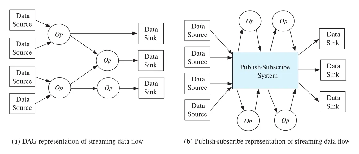 Figure 22.8 · PDF p. 1100 · streaming data flow를 DAG와 publish-subscribe 방식으로 표현한 routing 구조
Figure 22.8(a)의 DAG에서 Data Source nodes는 stream sources에서 tuples를 받아 system에 inject하는 entry points다. Data Sink nodes는 tuples가 system을 떠나는 exit points이며, output은 data store/file system에 저장되거나 외부로 전달될 수 있다. Apache Storm은 graph를 configuration으로 정의하며, 이를 topology라고 부른다. Storm terminology에서는 data source nodes를 spouts, operator nodes를 bolts라고 한다.
다른 방식은 publish-subscribe system, 줄여서 pub-sub system이다. Data는 topic과 함께 publish되고, subscribers는 관심 topics를 subscribe한다. Topic에 document/tuple이 publish되면 해당 topic subscribers에게 copy가 전달된다. Stream processing에서 tuple은 document처럼 취급되고, operators는 input topics를 subscribe하고 output topics로 publish한다.
Publish-subscribe 방식의 장점은 operators를 추가/제거하기 쉽다는 점이다. Figure 22.8(b)처럼 data source마다 unique topic name이 있고, operator output도 unique topic name을 가진다. Data sinks는 필요한 operator output topics를 subscribe한다.
Kafka는 publish-subscribe model을 사용한다. Kafka에서 topic에 publish된 tuples는 subscriber가 없어도 retention period 동안 보존된다. Subscriber processing이 failure 때문에 지연되거나 일시 중단되어도 retention time 안에서는 tuples를 다시 처리할 수 있다. Millwheel, Muppet 같은 systems는 topic 대신 stream이라는 용어를 사용한다.
Physical routing에서는 logical operator 하나가 여러 physical instances로 병렬 실행된다. Incoming tuples는 partitioning function에 따라 operator instances 중 하나 또는 여러 개로 보내진다. Kafka에서는 topic이 여러 topic-partitions로 나뉘고, tuple은 그중 하나로 간다. Tuple에 partition key를 붙이면 같은 key의 tuples가 같은 partition으로 전달되도록 보장할 수 있다.
Kafka의 consumer group은 logical operator에 해당하고, group 안의 individual consumers는 parallel physical instances다. Topic의 tuple 하나는 consumer group 안의 consumer 하나에게만 전달된다. 더 정확히는 topic-partition 하나의 tuples는 consumer group 안의 single consumer에게 가며, consumer 하나가 multiple partitions를 받을 수도 있다.
22.8.2 Parallel Processing of Stream Operations
Standard relational operations의 parallel evaluation 기법은 streaming data에도 적용된다. Selection/projection은 서로 다른 tuples에 대해 병렬 처리하기 쉽다. Grouping은 같은 group의 tuples를 한 machine으로 모아야 하므로 grouping key 기준 partitioning이 필요하다. Grouping + aggregation에서는 pre-aggregation으로 transfer volume을 줄일 수 있지만, group에 속한 정보는 결국 같은 machine에 도착해야 한다.
windowing은 streaming system의 핵심 operation이다. Incoming data를 timestamp 또는 tuple count 기준 windows로 나누고, window 안에서 grouping/aggregation을 수행한다. Window를 쓰면 system이 “이 window에 더 이상 new tuple이 들어오지 않는다”고 판단한 시점에 aggregate result를 output할 수 있다. 예를 들어 5-minute window라면, future tuples의 timestamp가 해당 window end보다 크다는 것이 확정되면 그 window aggregate를 내보낼 수 있다.
Windowing과 grouping을 함께 쓰고 windows가 overlap될 때는 partitioning key를 window까지 포함하지 않고 grouping attributes만 사용하는 것이 좋다. Tuple 하나가 multiple overlapping windows에 속할 수 있기 때문이다. Window까지 partitioning하면 같은 tuple을 여러 windows/nodes로 보내는 overhead가 생긴다.
User-defined operators도 parallelize되어야 한다. 보통 각 tuple에 key를 붙이고, 같은 key의 tuples는 같은 operator instance로 보낸다. Different keys는 different instances로 보내 parallel processing한다. 이 방식은 key별 state consistency를 유지하면서 scale-out을 가능하게 한다.
Stream operators는 state를 저장하는 경우가 많다. Window operator는 active window의 tuples 또는 per-minute aggregates 같은 intermediate state를 유지할 수 있고, user-defined operators도 local variables/state를 가진다. State 저장 위치에는 trade-off가 있다.
| State 저장 방식 | 장점 | 위험 |
|---|---|---|
| Local node state | 접근 비용이 낮고 latency가 작다. | Node failure 시 state loss 위험이 크다. |
| Parallel data-storage system | Replication/high availability를 이용할 수 있다. | Access/update cost가 커지고 latency가 증가할 수 있다. |
22.8.3 Fault Tolerance with Streaming Data
Stored data query는 failure가 나면 query 전체 또는 일부를 reexecute할 수 있다. Streaming setting에서는 이 방식이 어렵다. Streaming applications는 latency sensitive하고, continuous outputs를 내보내므로 restart/reexecution이 duplicate outputs를 만들 수 있다.
Streaming systems는 output delivery semantics를 명확히 해야 한다.
| Semantics | 보장 | 문제 |
|---|---|---|
at-least-once | 각 tuple이 최소 한 번 output된다. | Recovery 중 duplicate delivery가 가능하다. |
at-most-once | 각 tuple이 최대 한 번 output된다. | Failure 시 tuple loss가 가능하다. |
exactly-once | Failure와 무관하게 각 tuple이 정확히 한 번 output된다. | 구현 비용이 가장 크지만 대부분 applications가 원하는 semantics다. |
이 semantics를 보장하려면 각 operator가 어떤 input tuples를 처리했고 어떤 output tuples를 냈는지 추적해야 한다. Duplicate 제거는 normal processing 중 duplicate가 없다는 전제에서만 query semantics를 해치지 않는다. 원래 의미상 duplicate가 가능한 stream에서 무조건 제거하면 잘못된 결과가 된다.
Fault tolerance는 routing subsystem이 제공할 수도 있다. Kafka는 topic-partition을 둘 이상의 nodes에 저장하고, 각 node에서 tuples를 disk에 기록한다. 그래서 node failure나 restart에도 tuples가 사라지지 않는다. Stream processing system은 이 lower-level availability를 이용해 higher-level operator recovery를 구현할 수 있다.
Operator가 failed node에서 실행 중이었다면 다른 node에서 restart할 수 있다. System은 각 input stream을 어디까지 소비했는지, 즉 offset/progress를 주기적으로 기록해야 한다. Stateless operator는 적절한 point부터 input stream을 replay하면 된다. Stateful operator는 failure 전 state도 복구해야 하므로 더 어렵다. Window operator는 window start에 해당하는 point부터 replay하거나, 큰 window라면 checkpoint를 사용해야 한다.
Stateful streaming recovery의 일반 패턴은 다음과 같다.
- Operator state와 input stream progress를 periodic checkpoint로 저장한다.
- Failure가 발생하면 latest checkpoint를 restore한다.
- Last checkpoint 이후 처리된 stream tuples만 replay한다.
- Checkpointed state는 local storage보다 distributed file system 또는 parallel data-storage system에 저장하면 failed node 없이도 recovery를 계속할 수 있다.
Underlying routing system이 fault tolerance를 제공하지 않으면 operator가 직접 output tuples를 보존해야 한다. 어떤 tuple이 consumer에게 더 이상 필요 없다는 것을 알기 전까지 discard하지 않는 식이다.
Low-latency failure handling을 위해 일부 streaming systems는 operator replicas를 동시에 실행한다. 하나는 primary copy, 다른 하나는 hot-spare replica로 두고, primary failure 시 spare output을 사용한다. 이때 replicas가 만든 duplicate tuples가 consumers에게 중복 전달되지 않도록 system이 조정해야 한다.
22.9 Distributed Query Processing
Distributed query processing은 원래 geographically distributed databases를 대상으로 queries를 실행해야 하는 필요에서 출발했다. 오늘날에는 같은 조직 안에서도 data가 multiple databases, data storage systems, files, cloud services에 흩어져 있기 때문에 같은 문제가 더 일반적으로 등장한다.
22.9.1 Data Integration from Multiple Data Sources
Enterprise의 부서별 systems, merger로 합쳐진 systems, legacy applications는 서로 다른 DBMS와 schemas를 사용할 수 있다. 모든 data를 하나의 common system으로 migration하는 것은 비싸고 시간이 오래 걸린다. 대안은 각 data를 원래 위치에 두되, 사용자에게는 integrated logical view를 제공하는 것이다.
이때 local systems는 서로 다른 logical models, data-definition languages, data-manipulation languages, concurrency-control/transaction-management mechanisms를 가질 수 있다. 일부 source는 full DBMS가 아니라 key-value data storage, files, web service일 수도 있다. 따라서 기존 systems 위에 integration software layer가 필요하다. 이 layer가 physical integration 없이 logical integration illusion을 제공하면 federated database system이라고 부른다.
Data integration 접근은 다음과 같다.
| 접근 | 핵심 | 장점/한계 |
|---|---|---|
federated database approach | 모든 sources 위에 common global schema를 만든다. 각 database는 local schema를 유지한다. | Users는 global schema에 query하지만, query/update를 local schemas로 translate해야 한다. |
mediator system | Common schema query는 지원하지만 update는 지원하지 않는 federation variant다. | Read integration에는 유용하지만 write semantics는 제한된다. |
data virtualization | Common schema를 강제하지 않고 multiple sources 접근과 combine을 숨긴다. | Users가 서로 다른 schemas를 알아야 할 수 있다. |
external data / foreign tables | DBMS 안에 external source의 schema, connection, authorization 정보를 등록한다. | Local table처럼 read/update할 수 있지만 supported operations는 source capabilities에 의존한다. |
SQL source는 ODBC/JDBC로 접근할 수 있고, HBase 같은 non-SQL parallel data storage는 해당 API로 접근한다. wrapper는 data source의 data를 원하는 schema로 보여주는 layer다. Wrapper는 global schema query를 local schema query로 translate하고, results를 다시 global schema로 translate한다. Nonrelational sources, 예를 들어 web services, flat files, directory systems도 wrapper를 통해 relational view로 노출될 수 있다.
Decision support query만 목표라면 data warehouse가 integration의 대안이다. Multiple sources에서 data를 periodic 또는 continuous import하고, clean/transform한 뒤 centralized schema로 저장한다. Warehouse는 source systems 부하를 줄이고 query processing을 효율적으로 만들지만, source update와 warehouse import 사이 delay 때문에 most recent data를 즉시 보지 못할 수 있다.
data lake는 data를 여러 storage systems와 formats에 그대로 두되, single system에서 query할 수 있게 하는 architecture다. Warehouse처럼 upfront preprocessing을 강제하지 않으므로 ingestion은 유연하지만, query 작성 시 schema/format 이해와 정제 부담이 커질 수 있다.
22.9.2 Schema and Data Integration
Unified view를 제공하려면 먼저 schema integration이 필요하다. 각 local system은 자기 conceptual schema를 갖고, integration system은 이를 하나의 global conceptual schema로 통합해야 한다. 가장 어려운 부분은 semantic heterogeneity다. 같은 attribute name이 다른 local databases에서 다른 의미를 가질 수 있고, 반대로 같은 의미가 다른 이름으로 표현될 수도 있다.
Schema integration은 두 가지 mapping 정보를 필요로 한다.
- Unified
global schema - Local schema data를 global schema representation으로 변환하는 mapping
global-as-view (GAV)는 global schema relation을 local sites의 views union으로 정의한다. 예를 들어 global student(ID, name, dept_name, tot_cred)가 있고, site s1은 student1(ID, name, dept_name)과 studentCreds(ID, tot_cred)를 저장하며, site s2는 student2(ID, name, tot_cred)와 studentDept(ID, dept_name)를 저장한다고 하자. 각 site는 local join으로 global student 형태의 view를 만들고, global student는 student_s1 union student_s2로 정의된다.
GAV는 global query를 local schema queries로 rewrite하기 쉽다. 하지만 global schema update를 local updates로 translate하는 것은 view update problem 때문에 어렵다. 어떤 global update가 local base tables에 유일하게 대응되지 않을 수 있기 때문이다.
local-as-view (LAV)는 반대로 local data를 global conceptual relation 위의 view로 정의한다. 예를 들어 student_s3는 global student 중 dept_name = 'Comp. Sci.'인 tuples, student_s4는 그 외 departments tuples라고 정의할 수 있다. 그러면 optimizer는 dept_name='Comp. Sci.' selection query를 site s3에만 보내고 s4를 건너뛸 수 있다.
Data integration에는 schema뿐 아니라 values/types 통합도 필요하다.
| 문제 | 예 | 해결 방향 |
|---|---|---|
| Type mismatch | 한 system의 type을 다른 system이 지원하지 않음 | View mapping에서 type conversion |
| Representation mismatch | ASCII vs Unicode, big-endian vs little-endian, floating-point representation 차이 | 공통 representation으로 변환 |
| Unit mismatch | length가 한 system에서는 inches, 다른 system에서는 millimeters | Semantic conversion rule 적용 |
| Name mismatch | Cologne vs Koeln처럼 같은 entity의 다른 이름 | globally unique naming system 또는 name equivalence mapping |
Linked Data처럼 RDF 기반 data integration에서는 equivalence를 명시할 수 있지만, equivalences가 많아질수록 query processing이 복잡해진다. View definitions는 virtual global view를 제공할 수도 있고, materialized global schema를 만들어 data warehouse로 저장할 수도 있다. 후자의 경우 underlying data updates를 warehouse로 propagate해야 한다.
22.9.3 Query Processing Across Multiple Data Sources
Multiple data sources query를 naive하게 처리하려면 필요한 data를 모두 query issuing site로 가져와 local query를 실행하면 된다. 하지만 selection condition으로 몇 records만 필요한데 large relation 전체를 가져오는 것은 낭비다. Source가 selection을 수행할 수 있다면 source에서 selection을 push down하고, 필요한 result만 가져와야 한다.
각 source의 query capability는 다를 수 있다. SQL DBMS는 selection, join, aggregation을 source에서 수행할 수 있지만, key-value store는 key attributes selection만 지원할 수 있고, web source는 특정 fields에 selection이 반드시 포함되어야 할 수도 있다. 따라서 query는 source에서 할 수 있는 부분과 issuing site에서 해야 하는 부분으로 나뉜다.
Cost는 local execution cost와 data transfer cost의 합이다. Wide-area network가 low bandwidth이면 data transfer minimization이 특히 중요하다.
22.9.3.1 Join Locations and Join Ordering
Expression r1 ⋈ r2 ⋈ r3에서 r1, r2, r3가 각각 sites S1, S2, S3에 있고 query result는 issuing site SI에 필요하다고 하자. 가능한 전략은 많다.
| 전략 | 설명 | 비용 고려 |
|---|---|---|
Ship all to SI | 세 relations를 모두 SI로 보내 local query processing한다. | Simple하지만 data shipping이 클 수 있고 source indices를 활용하지 못할 수 있다. |
| Move intermediate joins | r1을 S2로 보내 r1 ⋈ r2를 계산하고, intermediate result를 S3로 보내 r3와 join한 뒤 result를 SI로 보낸다. | Intermediate result size와 site별 processing speed에 따라 유리할 수 있다. |
| Alternative join order/site | Join order와 execution site를 바꾼 여러 variants | Network block transfer cost, local indices, source speed를 함께 고려해야 한다. |
No one strategy is always best. Optimizer는 intermediate result sizes, network transmission costs, each site processing costs, useful indices availability를 기준으로 strategy를 선택해야 한다.
22.9.3.2 Semijoin Strategy
semijoin strategy는 distributed join에서 shipping data를 줄이기 위한 핵심 기법이다. r1은 site S1, r2는 site S2에 있고 result는 S1에 필요하다고 하자. r2의 많은 tuples가 r1과 join되지 않는다면 r2 전체를 S1으로 보내는 것은 낭비다.
Natural join attributes가 R1 ∩ R2일 때 전략은 다음과 같다.
S1에서temp1 <- ΠR1∩R2(r1)를 계산한다.temp1을S2로 보낸다.S2에서temp2 <- r2 ⋈ temp1을 계산한다. 이는r2중r1과 join 가능성이 있는 tuples만 남기는 효과다.temp2를S1으로 보낸다.S1에서r1 ⋈ temp2를 계산해 final result를 얻는다.
Semijoin은 다음처럼 정의된다.
Theta semijoin도 가능하다.
Semijoin strategy는 r2 중 실제 join에 참여하는 fraction이 작을 때 특히 유리하다. 추가 비용은 temp1을 S1에서 S2로 보내는 것이다. 이 비용보다 r2 전체 대신 r2 ⋉ r1만 보내는 절감이 크면 semijoin이 이득이다.
Bloom filter는 semijoin의 efficient overapproximation을 만든다. r1의 join attributes를 hash해 bitmap bits를 set하고, bitmap만 S2로 보낸다. S2는 r2 tuples의 join attribute를 같은 hash function으로 검사해 bit가 1인 tuples만 보낸다. Bloom filter는 false negative가 없어야 한다. 즉, 실제 join될 tuple은 절대 버리면 안 된다. 대신 false positive는 허용된다. False positive로 extra r2 tuples가 S1에 가더라도 final join에서 제거된다.
False positive rate를 낮추려면 bitmap size를 distinct join attribute values 수보다 몇 배 크게 잡고, 여러 independent hash functions를 사용한다. 원문 예시처럼 bitmap이 10n bits이고 distinct values가 n, hash functions가 k=7이면 false positive rate가 약 1%가 될 수 있다.
22.9.3.3 Distributed Query Optimization
Distributed query optimization은 기존 optimizer에 다음 확장을 요구한다.
| 확장 | 의미 |
|---|---|
| Data location as physical property | Sort order처럼 data location도 physical property로 추적한다. Site가 맞지 않으면 exchange/data transfer가 필요하다. |
| Operator execution site choice | Hash join/merge join 같은 algorithm 선택뿐 아니라, 어느 site에서 operator를 실행할지도 선택한다. |
| Semijoin transformations | Data transfer를 줄이기 위해 semijoin을 logical transformation으로 고려한다. Search space 폭발을 막기 위해 base tables에만 적용하는 heuristic을 쓸 수 있다. |
| Schema information pruning | LAV처럼 data partitioning semantics가 있으면 관련 없는 sites를 query execution에서 제외한다. |
예를 들어 student가 dept_name='Comp. Sci.' tuples는 site s3, 나머지는 site s4에 있다고 LAV로 알려져 있으면, dept_name='Comp. Sci.' query는 s4에 보낼 필요가 없다. 또 site s5가 s3의 replica라면 optimizer는 둘 중 더 싼 site를 선택하면 되고 둘 다 실행할 필요는 없다.
22.9.4 Distributed Directory Systems
directory는 persons, machines, organizational units 같은 객체 class에 대한 정보를 담은 listing이다. Directory는 특정 object 정보를 찾거나, 반대로 조건을 만족하는 objects를 찾는 데 쓰인다. 여러 directory access protocols는 directory data 접근을 표준화한다.
대표적인 distributed directory system은 DNS (Domain Name Service)다. DNS는 db-book.com, www.cs.yale.edu 같은 domain names를 IP addresses로 mapping한다. Network는 실제로 IP address로 messages를 route하므로, domain name을 IP address로 변환하는 service는 internet 동작에 필수다. LDAP (Lightweight Directory Access Protocol)은 organizational data 저장과 접근에 널리 쓰이는 protocol이다.
Directory data도 relational model로 표현하고 JDBC/ODBC로 접근할 수 있는데, 왜 별도 directory protocol이 필요한가? 이유는 다음과 같다.
| 이유 | 설명 |
|---|---|
| Limited access에 맞춘 단순 protocol | Directory access는 일반 DBMS query보다 제한된 pattern이 많다. |
| Hierarchical naming | File system directory처럼 hierarchical names가 중요하다. 예: cs.yale.edu, math.yale.edu. |
| Distributed hierarchical control | 각 organization/domain이 자기 subdomain data를 저장·관리한다. |
| Automatic forwarding | Query가 제출된 site에서 실제 data가 있는 site로 자동 전달되어 unified view를 제공한다. |
| Replication | Directory data availability를 위해 replicas를 유지한다. |
LDAP 기반 directory systems는 employees의 identifier, name, email, organization unit, room number, phone number, encrypted password 등을 저장하고 authentication에 사용된다. 오늘날에는 storage 자체가 centralized되거나 relational DBMS를 backend로 쓰는 directory implementation도 많지만, standardized data representation과 access protocol 덕분에 계속 널리 쓰인다.
22.10 Summary
Chapter 22의 큰 흐름은 data parallelism을 query processing 전체로 확장하는 것이다. Sort, join, selection, duplicate elimination, projection, aggregation은 exchange와 local operator 조합으로 parallelize된다. exchange operator는 hash/range partitioning, broadcasting, collect, merge를 담당하고, local operators는 centralized DBMS처럼 실행된다.
Parallel query processing의 성능은 단순히 CPU를 많이 쓰는 문제가 아니다. Data redistribution, network bandwidth, skew, startup cost, pipelining/materialization boundary, fault tolerance, shared-memory/NUMA/cache behavior가 모두 response time을 좌우한다.
Streaming data에서는 tuple routing과 delivery semantics가 핵심이다. DAG 또는 publish-subscribe model로 logical routing을 표현하고, physical instances로 parallel execution한다. exactly-once semantics를 제공하려면 progress tracking, checkpointing, replay, duplicate suppression이 필요하다.
Distributed query processing에서는 data가 multiple data sources에 흩어져 있으므로 schema/data integration과 query decomposition이 필요하다. Federated database, data virtualization, external data/foreign tables, wrappers, data warehouse, data lake는 서로 다른 integration trade-off를 가진다. Distributed joins에서는 join location/order와 semijoin/Bloom filter가 data transfer를 줄이는 핵심 도구다.
연결 관계
- Chapter 10: MapReduce, Spark, streaming concepts가 parallel execution과 fault tolerance의 실제 프레임워크 배경이 된다.
- Chapter 11: data warehouse와 data lake 논의가 distributed data integration의 대안으로 다시 등장한다.
- Chapter 14-16: B+-tree/hash join/sort/aggregation/query optimization이 parallel operator와 parallel optimizer의 기반이다.
- Chapter 20-21: shared-nothing/shared-memory architectures, partitioning, replication, skew, distributed file systems가 query execution의 물리적 기반이다.
- Chapter 23: distributed transactions, weak consistency, consensus, view consistency가 parallel materialized view maintenance와 distributed update semantics로 이어진다.
- Chapter 24: Bloom filter가 semijoin filtering의 핵심 probabilistic data structure로 다시 등장한다.
오해하기 쉬운 내용
interquery parallelism은 throughput을 높이는 데 좋지만 single query response time을 줄이지 않는다. Long analytical query에는intraquery parallelism이 필요하다.pipelined parallelism은 parallelism 자체보다 intermediate result materialization을 피하는 효과가 더 중요할 때가 많다.partitioned join은 equi-join에는 자연스럽지만 arbitrary inequality join에는 충분하지 않다. 이 경우 fragment-and-replicate가 필요할 수 있다.broadcast join은 항상 나쁜 replication이 아니다. Small relation을 broadcast하면 large relation repartition보다 훨씬 싸다.exchange operator는 단순 network send가 아니라 partitioning과 destination merge를 포함한 query-plan operator다.- Fault tolerance를 위해 materialize하면 recovery는 쉬워지지만 pipelining이 깨져 latency가 늘어난다.
exactly-once semantics는 output 중복 제거만으로 끝나지 않는다. State, input progress, replay boundary가 함께 맞아야 한다.GAV는 global query rewriting이 쉽지만 update translation이 어렵고,LAV는 data location/pruning 정보를 더 표현할 수 있지만 query rewriting이 복잡해질 수 있다.- Bloom filter semijoin은 false positive를 허용하지만 false negative는 허용하지 않는다.
면접 질문
interquery parallelism,intraquery parallelism,intraoperation parallelism,interoperation parallelism을 예와 함께 구분하라.range-partitioning sort와parallel external sort-merge의 차이와 skew 위험을 설명하라.partitioned join이 equi-join에서 동작하는 이유와 non-equi join에서 한계가 생기는 이유를 설명하라.broadcast join이 좋은 선택이 되는 조건은 무엇인가?work stealing이 shared-memory system에서 shared-nothing보다 저렴한 이유는 무엇인가?exchange operator model이 기존 centralized query engine 재사용에 왜 유리한가?resource consumption cost model과response-time cost model의 차이를 예로 설명하라.- Parallel query optimizer가 partitioning을 physical property로 다루어야 하는 이유는 무엇인가?
- Streaming system에서
at-least-once,at-most-once,exactly-oncesemantics를 비교하라. - Distributed join에서
semijoin strategy와Bloom filter가 data transfer를 줄이는 방식을 설명하라. global-as-view (GAV)와local-as-view (LAV)의 차이를 query rewriting과 update 관점에서 설명하라.- DNS와 LDAP가 distributed directory systems로 분류되는 이유를 설명하라.
용어 회수
parallel query processing, interquery parallelism, intraquery parallelism, intraoperation parallelism, interoperation parallelism, data parallelism, shared-nothing architecture, shared-memory architecture, range-partitioning sort, parallel external sort-merge, partitioned join, partitioned parallel hash join, partitioned parallel merge join, partitioned parallel nested-loop join, partitioned parallel indexed nested-loops join, fragment-and-replicate join, asymmetric fragment-and-replicate join, broadcast join, symmetric fragment-and-replicate join, join skew avoidance, dynamic handling of join skew, work stealing, parallel selection, parallel duplicate elimination, parallel projection, parallel aggregation, partial aggregation, MapReduce, map(), reduce(), intermediate key, combiner, pipelined parallelism, independent parallelism, push model, pull model, exchange operator, random merge, ordered merge, parallel query execution plan, straggler nodes, Resilient Distributed Datasets, RDD, threads, morsels, NUMA, Non-Uniform Memory Access, SIMD, Single Instruction Multiple Data, GPU, resource consumption cost model, response-time cost model, physical property, colocation of data, entity group, parallel view maintenance, materialized view, streaming data, lambda architecture, routing of streams, DAG, publish-subscribe, pub-sub, topic, topic-partition, consumer group, windowing, at-least-once semantics, at-most-once semantics, exactly-once semantics, checkpoint, hot-spare replica, distributed query processing, federated database system, global schema, local schema, schema integration, mediator system, data virtualization, external data, foreign tables, wrapper, data warehouse, data lake, global-as-view, GAV, local-as-view, LAV, Linked Data, semijoin strategy, semijoin, theta semijoin, Bloom filter, false positive, distributed directory system, DNS, Domain Name Service, LDAP, Lightweight Directory Access Protocol.