개요
Relational model은 많은 application domain에서 널리 쓰이지만, core relational model은 attribute value가 atomic해야 한다고 가정한다. 즉 multivalued, composite, nested, text, spatial 같은 complex data types는 기본 relational model 밖에 있다. Chapter 8은 이런 제약이 현실 application에서 오히려 부담이 되는 경우를 다룬다.
핵심 흐름은 “1NF/atomic domain이 단순하고 강력하지만, modern application은 더 복잡한 값을 자연스럽게 저장/교환/검색해야 한다”는 것이다. 그래서 semi-structured data, object orientation, textual data, spatial data가 등장한다.
핵심 개념
semi-structured data는 schema가 자주 바뀌거나 tuple마다 attribute 집합이 다른 data를 유연하게 표현한다.JSON(JavaScript Object Notation)과XML(Extensible Markup Language)은 nested structure를 가진 complex value를 text로 표현해 application 간 data exchange에 많이 쓰인다.RDF(Resource Description Framework)와knowledge graph는 entity, attribute, relationship을 triple 또는 graph로 표현한다.object orientation은 SQL/relational data에 object, type, inheritance, reference 개념을 결합하려는 흐름이다.textual data는 unstructured text를 keyword query, relevance ranking, TF-IDF, hyperlink 기반 ranking 같은 방식으로 검색한다.spatial data는 point, line, polygon, region, geographic object처럼 공간 정보를 저장하고 spatial predicate/query/index를 지원한다.
세부 정리
8.1 Semi-structured Data
Relational database design은 보통 fixed number of attributes를 가진 table을 만들고, 각 attribute에는 atomic value를 넣는다. Schema 변경은 드문 사건이고, 새 attribute를 추가하면 application code까지 바뀔 수 있다. 이런 방식은 payroll, banking, university registration처럼 안정적인 organizational application에는 잘 맞는다.
하지만 web/mobile application처럼 빠르게 변하는 domain에서는 schema가 자주 바뀌고, object 하나 안에 다양한 shape의 data가 들어갈 수 있다. 예를 들어 user profile은 application마다 필요한 attribute가 다르고, 시간이 지나면서 interests, preferences, settings, linked accounts 같은 attribute가 계속 추가될 수 있다. Interests처럼 set-valued data는 normalized relation으로 분리할 수도 있지만, 항상 user 단위로 읽는 workload라면 set data type으로 한 번에 가져오는 편이 훨씬 효율적일 수 있다.
Semi-structured data의 또 다른 큰 동기는 data exchange다. Modern information system은 backend web service가 data를 제공하고, mobile app 또는 browser JavaScript가 client side에서 responsive UI를 만든다. 이때 backend와 client 사이에서 complex data를 효율적으로 주고받아야 하므로 JSON/XML 같은 representation이 중요해졌다.
8.1.1 Overview of Semi-structured Data Models
Semi-structured data model은 relational model의 고정 schema/atomic value 가정을 여러 방향으로 확장한다.
| 확장 방향 | 핵심 아이디어 | 왜 필요한가 |
|---|---|---|
wide column data representation | tuple마다 서로 다른 attribute set을 가질 수 있음 | schema evolution이 잦은 data를 유연하게 저장 |
sparse column representation | 매우 많은 fixed attributes를 두고 필요한 것만 사용, 나머지는 null | tuple shape는 다양하지만 physical schema를 고정하고 싶을 때 |
multivalued data types | set, multiset, array를 attribute value로 저장 | nested/collection data를 join 없이 한 object 안에서 다룸 |
key-value map | key가 최대 한 번만 등장하는 (key, value) pair 집합 | product specification처럼 항목마다 다른 속성을 저장 |
nested data types | object 안에 sub-object, array, map을 포함 | business object 또는 application object의 계층 구조를 직접 표현 |
knowledge representation | facts와 relationships를 triple/graph로 표현 | web-scale knowledge base와 inference/query를 지원 |
wide column은 각 tuple이 서로 다른 attribute set을 가질 수 있다는 점에서 fixed relational table과 다르다. sparse column은 더 제한된 형태로, 매우 많은 attribute를 미리 만들고 실제 tuple은 일부만 사용한다. 둘 다 schema flexibility를 얻지만, attribute 의미와 질의 패턴을 application이 더 많이 관리해야 한다.
multivalued data types는 Chapter 7의 1NF와 직접 연결된다. Core relational model에서는 set-valued attribute를 별도 relation으로 정규화하지만, 항상 parent object 단위로 접근한다면 normalized representation은 storage/query overhead를 키울 수 있다. 예를 들어 user interests가 다음 set으로 저장될 수 있다.
{ basketball, La Liga, cooking, anime, Jazz }Product detail처럼 item마다 서로 다른 specification을 갖는 경우에는 map이 자연스럽다.
{ (brand, Apple), (ID, MacBook Air), (size, 13), (color, silver) }Map은 보통 put(key, value), get(key), delete(key) 같은 operation으로 다룬다. Array는 scientific image, sensor readings, monitoring data처럼 ordered/multidimensional data에서 중요하다. 일정 간격의 sensor readings를 (time, reading) tuple들로 저장하면 time 값과 tuple overhead가 반복된다. 반면 array로 저장하면 offset으로 time을 추론할 수 있고, compression을 적용하기도 쉽다.
이처럼 set/array/map을 relation attribute로 허용하는 model은 non first-normal-form(NFNF) data model이라고 불렸다. 오늘날 여러 relational database도 set/array type을 지원하고, array database는 compressed array storage와 array operation query extension을 전문적으로 제공한다.
nested data types는 composite attribute와 multivalued value를 계층적으로 결합한다. 예를 들어 name이 firstname, lastname을 component로 갖고, object가 children array를 포함할 수 있다. JSON/XML은 이런 nested data를 schema에 강하게 묶지 않고 표현한다. 한 object가 sub-object를 갖는 tree structure가 되므로, business object 하나를 document처럼 묶어 교환하거나 저장하기 좋다.
knowledge representation은 artificial intelligence와 web-scale knowledge base에서 온 흐름이다. RDF는 복잡한 rule system보다 단순하지만 큰 data volume을 다루기 좋아 널리 쓰인다. RDF는 data를 object, attribute, relationship으로 보고, triple 또는 graph로 표현한다.
8.1.2 JSON
JSON(JavaScript Object Notation)은 complex data type을 textual representation으로 표현하는 형식이다. Primitive type으로 integer, real, string을 지원하고, collection/structure로 array와 object를 지원한다. JSON object는 attribute name과 value의 pair 집합이므로 key-value map과 거의 같다.
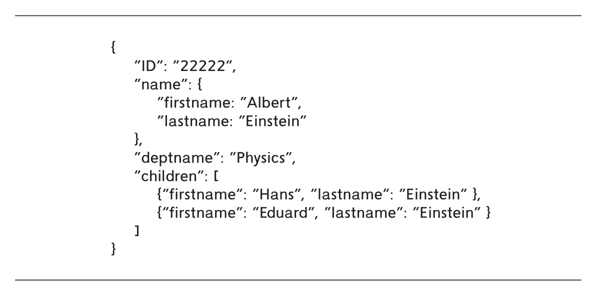 Figure 8.1 · PDF p. 398 · nested object와 array를 포함한 JSON data 예
Figure 8.1은 instructor-like object 안에 ID, nested name, deptname, children array가 함께 들어가는 모습을 보여준다. Relational representation이라면 name의 component와 children을 별도 relation으로 분해할 수 있지만, JSON은 application object에 가까운 구조를 그대로 문서 하나로 포장한다.
JSON array는 square brackets로 표현되며, integer offset에서 value로 가는 map처럼 생각할 수 있다. 이 특징 때문에 JSON은 application object와 언어의 in-memory data structure 사이를 오가기 쉽다. JavaScript, Java, Python, PHP 등 대부분의 언어가 JSON serialization/deserialization library를 제공한다.
JSON이 web service에서 널리 쓰이는 이유는 다음과 같다.
| 이유 | 설명 |
|---|---|
| Complex structure 표현 | nested object, array, primitive value를 한 representation에 담을 수 있다 |
| Flexible schema | object마다 attribute set과 type이 달라도 된다 |
| Client-server exchange에 적합 | backend API와 browser/mobile app 사이에서 data를 주고받기 쉽다 |
| Programming language와 연결 쉬움 | JSON object를 application object/map/list로 변환하기 쉽다 |
하지만 JSON은 relational representation보다 verbose하다. Attribute name이 반복되고 text parsing이 필요하므로 storage와 CPU cost가 커질 수 있다. 그래서 storage 목적에서는 compressed/binary representation이 자주 쓰인다. 대표적으로 BSON(Binary JSON)은 JSON data를 binary 형태로 저장해 parsing cost와 storage overhead를 줄인다.
SQL도 JSON을 다루도록 확장되었다. 세 가지 방향이 중요하다.
| SQL JSON 지원 | 의미 |
|---|---|
| JSON data type | JSON value를 column에 저장 |
| SQL result에서 JSON 생성 | relational rows를 JSON object/array로 포장 |
| JSON path extraction | JSON object 내부 field를 path로 추출 |
예를 들어 PostgreSQL의 json_build_object() 같은 함수는 query result row에서 JSON object를 만들고, json_agg 같은 aggregate는 여러 JSON object를 하나의 JSON array/object로 묶는다. JSON field extraction은 DBMS마다 syntax가 다르다. PostgreSQL은 v->'ID' 같은 operator를 쓰고, SQL Server는 JSON_VALUE(value, path) 같은 function을 사용한다. 중요한 점은 SQL 표준적 사고와 달리 JSON extension syntax/semantics가 DBMS별로 상당히 다르다는 것이다.
8.1.3 XML
XML(Extensible Markup Language)은 angle bracket < >로 둘러싼 tag를 사용해 text에 구조를 부여한다. Tag는 보통 시작 tag와 종료 tag의 pair로 사용된다.
<title>Database System Concepts</title>Relational data도 XML tag로 표현할 수 있다.
<course>
    <course id> CS-101 </course id>
    <title> Intro. to Computer Science </title>
    <dept name> Comp. Sci. </dept name>
    <credits> 4 </credits>
</course>
XML의 장점은 tag 이름 자체가 data의 의미를 드러내므로 어느 정도 self-documenting하다는 점이다. 또한 tag nesting으로 hierarchical structure를 만들 수 있다. Purchase order, bill, invoice처럼 하나의 business object가 여러 subpart를 포함하는 경우 XML document 하나로 자연스럽게 표현할 수 있다.
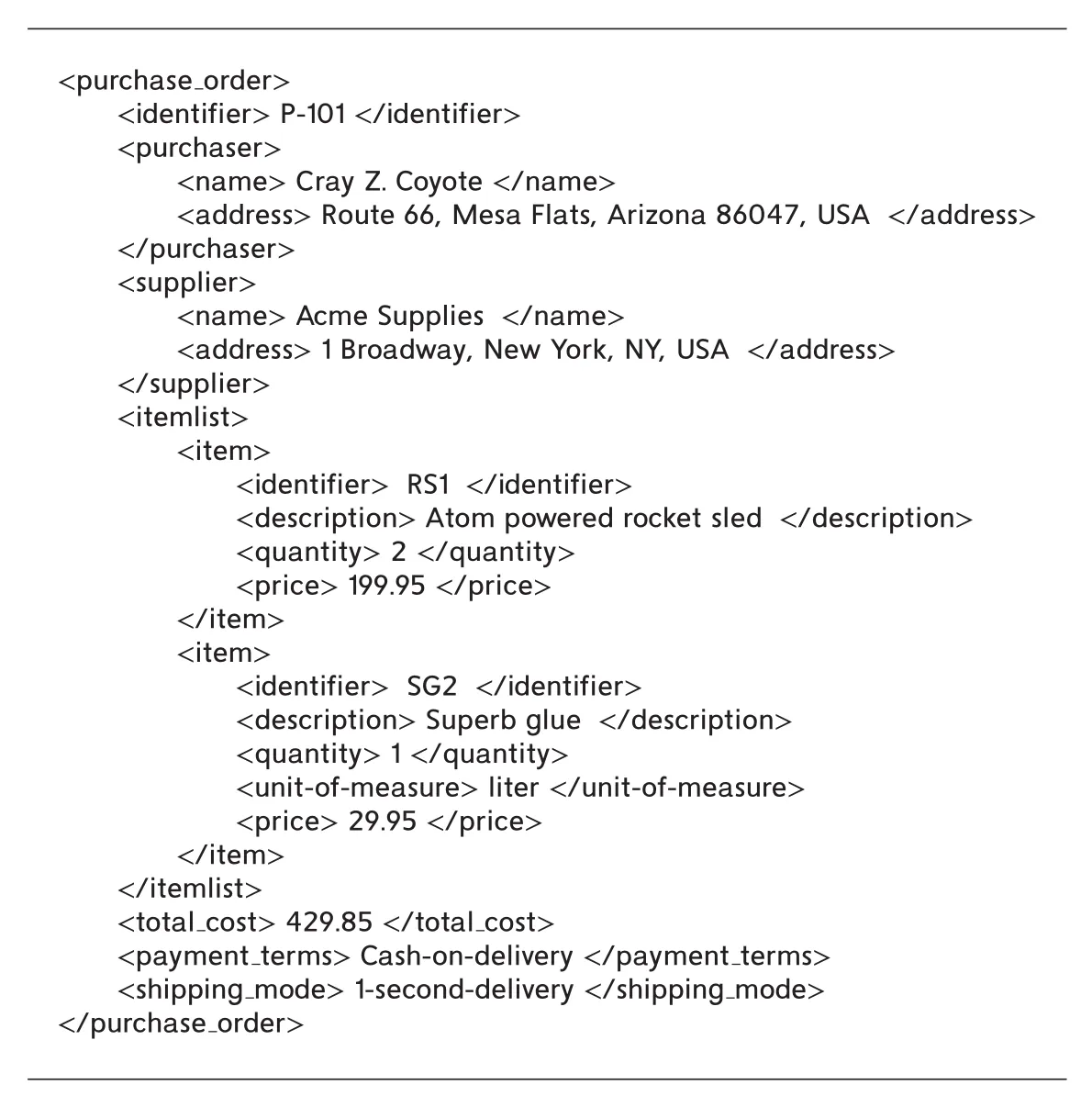 Figure 8.2 · PDF p. 400 · purchase order를 nested XML document로 표현한 예
Figure 8.2의 purchase order는 purchaser, supplier, itemlist, item, total cost, payment terms 같은 정보를 하나의 nested document로 담는다. 조직 간 data exchange에서는 양쪽이 어떤 tag가 어떤 의미인지 합의해야 한다.
XML query를 위해 XQuery가 개발되었지만, SQL만큼 널리 채택되지는 않았다. 대신 SQL 자체도 XML을 지원하도록 확장되었다.
| SQL XML 지원 | 의미 |
|---|---|
| XML data type | XML document/value를 column에 저장 |
| relational data에서 XML 생성 | query result를 XML document로 포장, XMLAGG 같은 aggregate 사용 |
| XML data extraction | XPath path expression으로 XML document 일부를 추출 |
JSON과 XML은 둘 다 nested semi-structured data를 표현하지만, 오늘날 application API exchange에서는 JSON이 더 일반적이고, XML은 configuration, legacy system, organization-to-organization document exchange에서 여전히 많이 보인다.
8.1.4 RDF and Knowledge Graphs
RDF(Resource Description Framework)는 E-R model과 비슷하게 object, attribute, relationship을 표현하지만, 더 단순한 triple representation을 사용한다. RDF에서 entity는 resource라고도 부른다.
RDF triple은 두 형태 중 하나다.
Triple의 세 위치는 각각 subject, predicate, object라고 부른다.
(subject, predicate, object)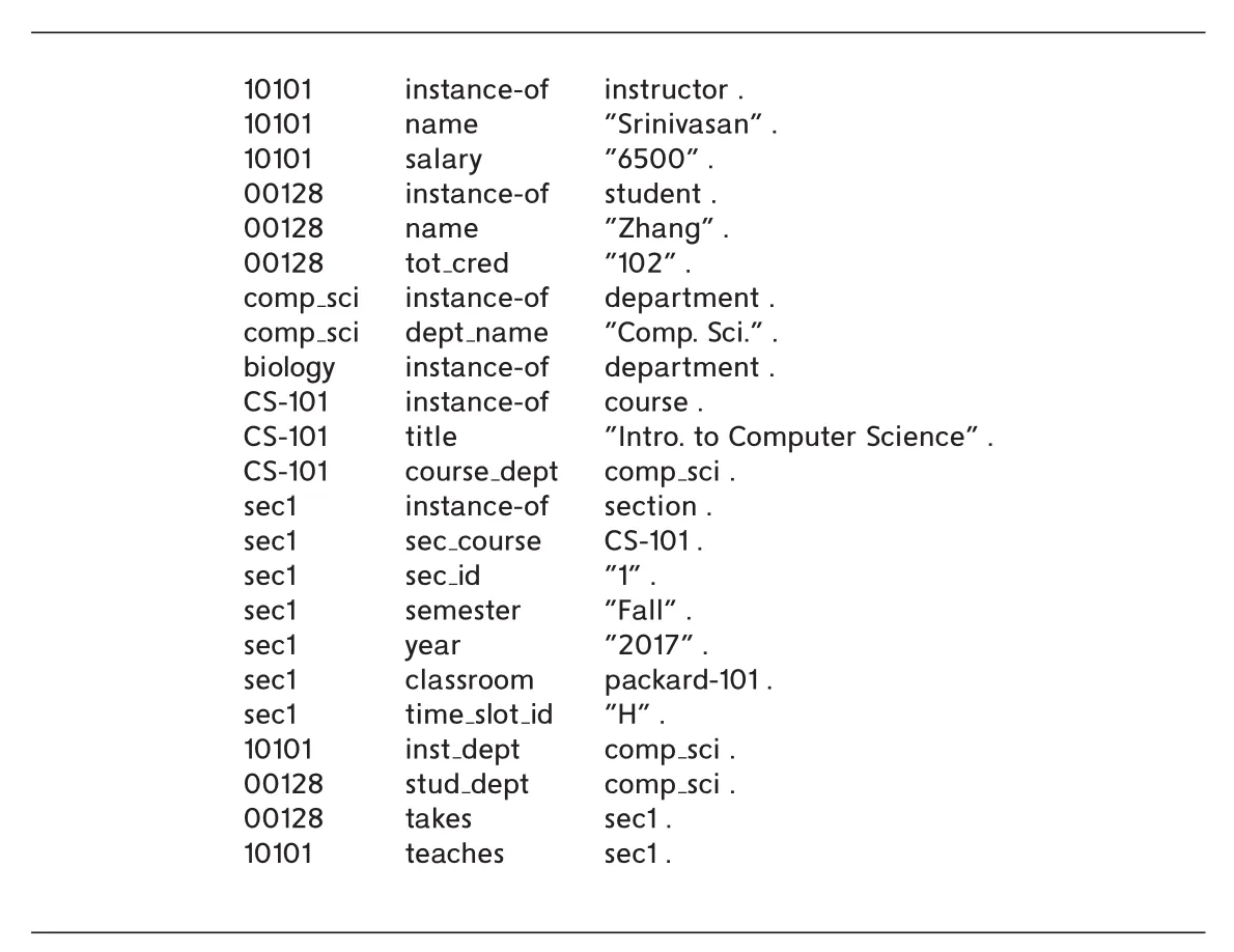 Figure 8.3 · PDF p. 402 · University database 일부를 RDF triple로 표현한 예
Figure 8.3은 instructor, student, department, course, section 정보를 triple로 표현한다. Attribute value는 quotes로 표시되고, object identifier는 quotes 없이 표시된다. instance-of relationship은 object의 type 정보를 제공한다. 예를 들어 10101 instance-of instructor는 ID 10101이 instructor instance임을 나타낸다.
RDF는 E-R model과 달리 기본적으로 binary relationship만 지원한다. N-ary relationship을 직접 표현하지 못한다는 한계가 있고, 뒤에서 reification/context/quads 같은 방식으로 보완한다.
RDF는 graph로 해석하기 매우 자연스럽다. Entity와 attribute value는 node가 되고, attribute name과 relationship name은 labeled edge가 된다.
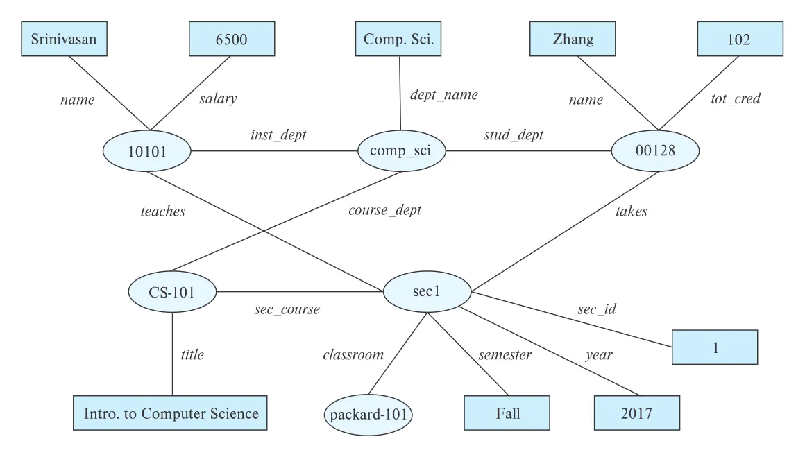 Figure 8.4 · PDF p. 403 · RDF triples를 node-edge graph로 해석한 knowledge graph
RDF graph model 또는 그 변형으로 표현된 정보 구조를 knowledge graph라고 부른다. Knowledge graph는 Wikipedia, Wikidata, web sources 등에서 수집한 fact를 저장하고 질의하는 데 쓰인다. 예를 들어 “Washington, D.C. is the capital of U.S.A.”는 capital-of edge로 두 entity를 연결하는 graph fact가 된다.
8.1.4.3 SPARQL
SPARQL은 RDF data를 질의하기 위한 query language다. 핵심은 triple pattern이다. Triple pattern은 RDF triple처럼 생겼지만 variable을 포함할 수 있다.
?cid title "Intro. to Computer Science"여기서 ?cid는 variable이고, predicate가 title, object가 "Intro. to Computer Science"인 모든 triple의 subject와 match된다.
여러 triple pattern은 shared variable을 통해 join된다.
?cid title "Intro. to Computer Science"
?sid course ?cid
첫 pattern이 course ID를 찾고, 두 번째 pattern이 그 course를 가진 section을 찾는다. Shared variable ?cid가 join condition 역할을 한다.
학생 이름을 찾는 SPARQL query는 다음처럼 구성된다.
select ?name
where {
    ?cid title "Intro. to Computer Science" .
    ?sid course ?cid .
    ?id takes ?sid .
    ?id name ?name .
}
SQL과 다른 중요한 특징은 triple pattern의 predicate 위치도 variable이 될 수 있다는 점이다. 즉 relationship/attribute name 자체를 질의의 일부로 variable match할 수 있다. SPARQL은 aggregation, optional joins, subqueries도 지원한다.
8.1.4.4 Representing N-ary Relationships
Knowledge graph의 edge는 기본적으로 binary relationship만 표현한다. 하지만 현실 fact는 time period, source, qualifier를 포함하는 n-ary relationship일 수 있다. 예를 들어 “Barack Obama was president of the U.S.A. from 2008 to 2016”은 person, country, role, start year, end year를 포함한다.
이를 표현하는 한 방법은 n-ary relationship tuple 자체를 artificial entity로 만드는 것이다.
e1 --person--> Obama
e1 --country--> U.S.A.
e1 --president-from--> 2008
e1 --president-till--> 2016
이 방식은 Chapter 6의 E-R aggregation과 비슷하다. RDF에서는 relationship을 entity처럼 다루는 이런 아이디어를 reification이라고 한다. 많은 knowledge graph에서는 edge에 붙는 valid time, source, confidence 같은 extra information을 qualifier로 취급한다.
다른 방식은 triple에 네 번째 attribute인 context를 추가해 quad를 저장하는 것이다. 기본 relationship은 여전히 binary이지만, context entity에 time period 같은 attribute를 연결할 수 있다.
Knowledge graph는 Wikidata, DBPedia, Freebase, Yago 같은 general knowledge base와 domain-specific knowledge graph에서 사용된다. linked open data 프로젝트는 독립적으로 만들어진 knowledge graph들을 공개하고 서로 link해, 여러 graph의 정보를 함께 추론할 수 있게 하는 것을 목표로 한다.
8.2 Object Orientation
object-relational data model은 relational data model에 richer type system을 붙인다. Complex data types, object orientation, inheritance, reference 같은 개념을 SQL/relational database 안으로 끌어들이려는 시도다. 목표는 relational foundation, 특히 declarative access를 유지하면서 modeling power를 높이는 것이다.
문제의 출발점은 impedance mismatch다. 많은 application은 Java, Python, C++ 같은 object-oriented programming language로 작성되지만, data는 relational database에 저장된다. Program 안의 object/type system과 database의 relation/tuple/type system이 다르기 때문에, fetch/store 때마다 변환이 필요하다. SQL이라는 별도 언어로 database access를 표현해야 하는 점도 programmer에게 부담이 된다.
Object orientation과 database를 결합하는 접근은 세 가지다.
| 접근 | 핵심 아이디어 | 장점 | 한계 |
|---|---|---|---|
object-relational database system | relational DBMS에 object-oriented features를 추가 | SQL/declarative query 기반을 유지하면서 type system 확장 | DBMS별 syntax와 feature support가 다름 |
object-relational mapping(ORM) | program object와 relational tuple 사이 mapping을 자동화 | programmer는 object model로 작업하고 DB는 relational로 유지 | bulk update/complex query에서 비효율 가능 |
object-oriented database system(OODB) | DBMS 자체가 object-oriented type system을 native 지원 | language integration이 좋음 | declarative querying 부족, pointer error로 corruption 위험, 상업적 성공 제한 |
원문은 object-oriented database approach를 길게 다루지 않는다. 이유는 명확하다. Database에서는 efficient access를 위해 declarative querying이 중요한데, imperative programming language는 이를 자연스럽게 제공하지 않는다. 또한 pointer를 통한 direct object access는 pointer error로 database corruption 위험을 높일 수 있다.
8.2.1 Object-Relational Database Systems
Object-relational DBMS는 relational system에 object-oriented feature를 추가한다. 대표적으로 user-defined types, type inheritance, table inheritance, reference types가 있다.
8.2.1.1 User-Defined Types
SQL의 object extension은 structured user-defined type(UDT)을 만들 수 있게 한다. 예를 들어 Person type을 만들고, 그 type의 tuple을 담는 people table을 만들 수 있다.
create type Person
    (ID varchar(20) primary key,
     name varchar(20),
     address varchar(20))
    ref from(ID);

create table people of Person;
이후 tuple은 일반 table처럼 insert할 수 있다.
insert into people (ID, name, address) values
    ('12345', 'Srinivasan', '23 Coyote Run');
UDT는 relation attribute의 type으로도 쓰일 수 있고, array/table type과 결합될 수 있다. 예를 들어 PostgreSQL은 integer[]처럼 크기가 미리 정해지지 않은 integer array를 지원하고, Oracle은 varray(10) of integer처럼 길이가 정해진 array syntax를 제공한다. SQL Server는 table-valued type을 정의할 수 있다.
create type interest as table (
    topic varchar(20),
    degree_of_interest int
);

create table users (
    ID varchar(20),
    name varchar(20),
    interests interest
);
이런 기능은 Chapter 8의 semi-structured data와 연결된다. Set/array/table-valued type을 relational table 안에 넣는 것은 core 1NF relational model보다 더 복잡한 value를 DBMS type system으로 직접 지원하는 방식이다.
8.2.1.2 Type Inheritance
type inheritance는 subtype이 supertype의 attributes와 methods를 물려받는 기능이다. Person type이 있고 student와 teacher가 person의 특수한 경우라면 다음처럼 정의할 수 있다.
create type Student under Person
    (degree varchar(20));

create type Teacher under Person
(salary integer);Student와 Teacher는 Person의 subtype이고, Person은 supertype이다. 두 subtype은 ID, name, address를 상속받고, 각각 degree, salary 같은 local attribute를 추가한다. Structured type에 method가 있다면 subtype도 이를 상속받을 수 있고, 경우에 따라 method behavior를 redefine할 수 있다.
8.2.1.3 Table Inheritance
table inheritance는 table 자체를 다른 table의 subtable로 선언하는 기능이다. E-R model의 specialization/generalization과 대응된다.
PostgreSQL 스타일로는 다음처럼 쓸 수 있다.
create table students
    (degree varchar(20))
    inherits people;

create table teachers
    (salary integer)
    inherits people;
이 경우 students, teachers table은 people의 attributes를 모두 가진다. Student tuple을 insert할 때는 inherited attributes와 local attributes 값을 함께 넣는다.
insert into student values
    ('00128', 'Zhang', '235 Coyote Run', 'Ph.D.');
Subtable의 중요한 의미는 tuple membership이다. students나 teachers에 있는 tuple은 implicitly people에도 존재하는 것으로 취급된다. 따라서 people을 query하면 people에 직접 inserted된 tuple뿐 아니라 subtables의 tuple도 함께 검색될 수 있다. 단, query가 접근할 수 있는 attribute는 people에 정의된 attributes로 제한된다. SQL은 only people 같은 표현으로 subtable tuple을 제외하고 supertable 자체 tuple만 검색할 수 있게 한다.
SQL:1999 방식에서는 먼저 table type을 정의하고, under people로 subtable을 만든다.
create table people of Person;
create table students of Student under people;
create table teachers of Teacher under people;
8.2.1.4 Reference Types in SQL
reference type은 어떤 tuple/object를 직접 참조하는 value를 저장하게 한다. 예를 들어 Department type이 department head를 Person에 대한 reference로 가질 수 있다.
create type Department (
    dept_name varchar(20),
    head ref(Person) scope people
);

create table departments of Department;
여기서 scope people은 departments.head가 people relation을 참조한다는 점을 명시한다. Foreign key의 역할을 reference type 문법으로 표현한다고 볼 수 있다.
Person type 정의에 ref from(ID)가 있으면, system-defined object identifier 대신 기존 primary key value인 ID를 reference로 사용할 수 있다. 그래서 다음 insert가 가능하다.
insert into departments values ('CS', '12345');System-generated reference를 쓰는 경우에는 ref(p)로 tuple reference를 얻고, update로 reference field를 채울 수 있다.
update departments
set head = (
    select ref(p)
    from people as p
    where ID = '12345'
)
where dept_name = 'CS';
Reference는 dereference해서 attribute에 접근할 수 있다. SQL:1999는 -> path expression을 사용한다.
select head->name, head->address
from departments;
또는 deref()로 reference가 가리키는 tuple을 얻은 뒤 attribute를 읽는다.
select deref(head).name
from departments;
Reference type의 장점은 join을 숨길 수 있다는 것이다. Reference가 없다면 department head의 name/address를 얻기 위해 departments와 people을 foreign key로 join해야 한다. Reference를 쓰면 query는 object navigation처럼 보인다. 다만 실제 DBMS 내부에서는 여전히 참조 무결성과 lookup 비용을 관리해야 한다.
8.2.2 Object-Relational Mapping
object-relational mapping(ORM)은 programming language의 object와 relational database의 tuples 사이 mapping을 정의한다. Programmer는 object를 retrieve/update/delete/create하는 방식으로 코드를 쓰고, ORM이 그 작업을 SQL query와 relational update로 변환한다.
ORM의 기본 동작 흐름은 다음과 같다.
Object query / selection condition
        ↓
ORM mapping
        ↓
SQL query over relational tables
        ↓
tuples retrieved from DB
        ↓
objects created in programming language
        ↓
object updates / new objects / delete marks
        ↓
save command
        ↓
insert / update / delete tuples in DB
ORM의 목표는 robust relational database의 장점을 유지하면서 application programmer에게 object model을 제공하는 것이다. Memory에 cache된 object를 다룰 때는 direct DB access보다 성능상 이득도 얻을 수 있다. 또한 ORM query language는 object model 위에서 작성되고, ORM이 이를 SQL로 translate한 뒤 result object를 만든다.
ORM의 장점과 비용은 함께 봐야 한다.
| 측면 | 장점 | 비용/주의점 |
|---|---|---|
| Programmer productivity | SQL을 직접 많이 쓰지 않고 object 중심으로 개발 | ORM mapping을 이해하지 못하면 비효율 query가 생김 |
| Portability | DBMS별 SQL 차이를 일정 부분 숨김 | DBMS 특화 feature를 쓰기 어려울 수 있음 |
| Caching | memory object cache로 repeated access 비용 감소 | stale data, transaction boundary 관리가 중요 |
| Complex query/bulk update | 필요하면 raw SQL로 우회 가능 | ORM만으로 작성하면 성능 비효율이 커질 수 있음 |
원문은 ORM이 많은 application에서 장점이 단점을 넘는다고 평가한다. Java의 Hibernate, Python의 Django ORM과 SQLAlchemy가 대표적이다. Chapter 9의 application architecture에서 ORM과 data-access layer가 다시 연결된다.
8.3 Textual Data
textual data는 unstructured text로 이루어진 data다. 이런 data를 질의하는 분야를 보통 information retrieval(IR)이라고 한다. IR의 전통적 model에서는 text information이 document 단위로 조직된다. Database에서는 text-valued attribute 하나를 document로 볼 수 있고, web에서는 web page 하나가 document가 된다.
8.3.1 Keyword Queries
Information retrieval system은 사용자가 원하는 information을 포함한 document를 찾아준다. 사용자는 보통 keyword query를 입력한다. 예를 들어 "database system"은 database system 관련 document를 찾기 위한 query이고, "stock", "scandal"은 stock-market scandal 관련 article을 찾기 위한 query가 될 수 있다.
가장 단순한 keyword query는 query의 모든 keyword를 포함하는 document를 반환한다. 하지만 실제 document collection이 크면 단순 반환만으로는 부족하다. 수십만 개 document가 match될 수 있으므로, system은 document가 query에 얼마나 관련 있는지 추정해 relevance ranking 순서로 보여줘야 한다.
Keyword는 text document뿐 아니라 image, video, audio 같은 data에도 적용된다. 이런 media object에 title, director, actor, genre, tag 같은 descriptive keyword가 붙어 있으면 keyword-based retrieval이 가능하다.
Web search engine도 핵심적으로는 information retrieval system이다. Web crawler가 web page를 수집해 저장하고, 사용자가 keyword query를 입력하면 keyword를 포함한 stored page를 찾는다. 다만 modern search engine은 단순 page retrieval을 넘어서 query의 topic을 판단하고, map, image, sports score, entity summary 같은 structured answer를 함께 보여준다. 즉 textual IR과 knowledge graph/structured data retrieval이 결합된다.
8.3.2 Relevance Ranking
Keyword를 포함하는 모든 document가 query에 똑같이 relevant한 것은 아니다. relevance ranking은 document가 query와 얼마나 관련 있는지 점수를 매기고, high-ranked documents만 먼저 보여주는 과정이다.
원문은 두 계열의 signal을 다룬다.
| ranking signal | 핵심 직관 |
|---|---|
| Keyword occurrence 기반 | query term이 document 안에서 얼마나 중요하게 등장하는가 |
| Hyperlink 기반 | web graph에서 document 자체가 얼마나 authoritative/popular한가 |
8.3.2.1 Ranking Using TF-IDF
term은 document 안에 등장하거나 query에 포함된 keyword다. 어떤 term t가 document d에 얼마나 relevant한지 측정할 때 단순 occurrence count만 쓰면 문제가 있다. 긴 document는 단어가 많이 나올 가능성이 높고, term이 10번 나온 document가 1번 나온 document보다 정확히 10배 relevant하다고 보기도 어렵다.
원문은 term frequency(TF)의 한 형태를 다음처럼 제시한다.
여기서 n(d)는 document d의 전체 term occurrence 수이고, n(d, t)는 document d에서 term t가 등장한 횟수다. 이 식은 document length를 고려하며, term occurrence가 많아질수록 relevance가 증가하지만 증가율은 logarithm 때문에 완만하다.
실제 system은 TF를 더 정교하게 만든다. Term이 title, author list, abstract에 있으면 더 중요하게 볼 수 있고, term의 첫 등장 위치가 늦으면 덜 relevant하게 볼 수 있다. IR 분야에서는 exact formula와 관계없이 document가 term에 대해 갖는 relevance component를 넓게 term frequency(TF)라고 부른다.
Query Q가 여러 keyword를 포함할 때는 각 term에 대한 relevance를 결합한다. 단순히 TF를 더하면 흔한 단어가 과도하게 영향력을 가질 수 있다. 예를 들어 "database"는 많은 document에 등장하지만 "Silberschatz"는 훨씬 드물다. "Silberschatz"를 포함한 document가 "database"만 포함한 document보다 query 의도에 더 가까울 수 있다.
이를 보정하는 값이 inverse document frequency(IDF)다.
n(t)는 indexed documents 중 term t를 포함하는 document 수다. Term이 흔할수록 IDF(t)가 작고, 드물수록 커진다.
Document d가 query term set Q에 대해 갖는 relevance는 다음처럼 계산할 수 있다.
사용자가 term별 weight w(t)를 지정할 수 있다면 TF(d, t)에 w(t)를 곱해 반영할 수 있다. 이런 방식이 TF-IDF ranking이다.
Text retrieval system은 보통 stop words도 제거한다. "and", "or", "a" 같은 매우 흔한 단어는 거의 모든 English document에 등장하므로 IDF가 극도로 낮고 query discrimination에 도움이 되지 않는다. System은 100개 안팎의 common words를 stop words로 정의하고 indexing/query에서 무시한다.
여러 term이 있는 query에서는 proximity도 중요하다. Query terms가 document 안에서 가까이 등장하면 서로 관련된 phrase/context일 가능성이 높으므로 더 높은 rank를 줄 수 있다.
정리하면 TF-IDF의 핵심 직관은 다음과 같다.
| 요소 | 점수에 미치는 효과 |
|---|---|
| term이 document 안에서 자주 등장 | relevance 증가 |
| document가 길어 단어 수가 많음 | 단순 count 효과를 보정 |
| term이 전체 collection에서 흔함 | IDF가 낮아져 영향 감소 |
| term이 rare함 | IDF가 높아져 영향 증가 |
| query terms가 가까이 등장 | phrase/context 관련성 증가 |
Information retrieval system은 r(d, Q)가 높은 document를 descending order로 반환한다. Relevant document가 너무 많기 때문에 보통 top-K result만 먼저 보여주고, 사용자가 필요하면 더 많은 result를 요청하게 한다.
8.3.2.2 Ranking Using Hyperlinks
Web에서는 document 내부 text만 보는 것이 아니라 hyperlink graph도 ranking에 사용한다. 많은 page에서 link된 page는 더 important하다고 볼 수 있고, important page에서 link된 page도 더 important하다고 볼 수 있다.
PageRank는 Google이 도입한 page popularity measure다. 기본 아이디어는 random walker가 hyperlink를 따라 web을 이동할 때 어떤 page에 있을 확률이 높은지를 page importance로 보는 것이다. PageRank는 query와 독립적인 static score이며, keyword query가 들어오면 TF-IDF 같은 content-based score와 결합해 최종 ranking에 사용된다.
Web pages에 integer identifier를 부여하고, T[i, j]를 page i에서 outgoing link를 따라 page j로 이동할 probability라고 하자. Page i의 outgoing link 수가 Ni이고 link를 균등하게 고른다면 다음과 같다.
PageRank P[j]는 다음 linear equation으로 정의된다.
여기서 N은 page 수이고, δ는 보통 0.15 정도로 둔다. δ / N은 random jump를 나타낸다. 사용자가 link만 따라가지 않고 임의의 page로 이동할 가능성을 모델링해, graph sink나 disconnected component 문제를 완화한다.
PageRank는 보통 iterative technique으로 푼다.
initialize P[i] = 1 / N for all pages
repeat
    compute new P[j] from old P[i] values
until max change in any P[i] is below cutoff
Hyperlink ranking에서 추가로 쓰이는 signal도 있다. Page visit frequency, search result에 표시되었을 때 click된 비율, hyperlink의 anchor text에 등장한 keyword 등이 relevance estimation에 반영된다. Anchor text의 keyword는 destination page가 어떤 내용인지 외부 page가 설명해 주는 신호이므로 높은 term frequency처럼 취급될 수 있다.
8.3.3 Measuring Retrieval Effectiveness
Ranking quality는 exact science가 아니다. 그래도 IR system의 검색 성능은 주로 precision과 recall로 측정한다.
| metric | 의미 |
|---|---|
precision | retrieved documents 중 실제 relevant documents의 비율 |
recall | 전체 relevant documents 중 system이 retrieved한 documents의 비율 |
Search engine에서는 answer가 매우 많고 사용자가 보통 상위 10개 또는 20개만 보기 때문에 precision@K, recall@K처럼 측정한다. 예를 들어 precision@10은 사용자가 본 top 10 result 중 relevant result 비율을 의미한다.
8.3.4 Keyword Querying on Structured Data and Knowledge Graphs
Structured data는 SQL 같은 query language로 질의하는 것이 일반적이다. 하지만 일반 사용자는 schema를 모르거나 SQL을 작성하기 어렵다. 그래서 keyword query를 structured/semi-structured data에 적용하는 기법이 연구되었다.
한 접근은 structured data를 graph로 표현하는 것이다. Tuple을 node로 보고, foreign key나 다른 connection을 edge로 본다. Keyword query는 keyword가 등장하는 tuple들을 찾고, 그 tuple들을 연결하는 path를 graph에서 찾는 문제로 바뀐다.
예를 들어 university database에서 "Zhang Katz"라는 query가 들어오면, system은 Zhang이 student tuple에 있고 Katz가 instructor tuple에 있음을 찾을 수 있다. 그리고 두 tuple이 advisor relation을 통해 연결되는 path, 또는 Zhang이 Katz가 가르치는 course를 수강한 path를 answer로 제시할 수 있다.
이런 query는 완전히 정의된 SQL query가 아니므로 다양한 종류의 answer가 가능하다. 따라서 path length, edge direction, edge weight, tuple popularity rank 등을 사용해 answer를 rank해야 한다.
Knowledge graph와 textual information도 함께 사용된다. 예를 들어 text document의 “Stonebraker developed PostgreSQL”에서 Stonebraker가 database researcher Michael Stonebraker를 가리킨다고 annotate할 수 있다. Knowledge graph가 그가 Turing award를 수상했다는 fact를 알고 있다면, "turing award postgresql" query에 대해 document text와 knowledge graph fact를 결합해 answer할 수 있다.
Modern web search engine은 crawled documents와 large knowledge graph를 함께 사용해 user query에 답한다. 이 지점에서 Chapter 8의 semi-structured data, RDF/knowledge graph, textual retrieval은 서로 연결된다.
8.4 Spatial Data
spatial data support는 location을 기준으로 data를 저장, indexing, querying해야 하는 application에서 중요하다. 원문은 spatial data를 크게 두 종류로 나눈다.
| 종류 | 좌표/공간 | 예 |
|---|---|---|
geographic data | round-earth coordinate system, latitude/longitude/elevation | road map, land-use map, topographic elevation map, political boundary, land ownership map |
geometric data | 2D/3D Euclidean space, X/Y/Z coordinates | building, car, aircraft, CAD object, physical design |
Geographic information system(GIS)은 geographic data 저장에 특화된 database system이다. 많은 DBMS가 geographic/geometric type을 지원한다. 예로 Oracle Spatial and Graph, PostGIS, SQL Server, IBM DB2 Spatial Extender 등이 있다. 단, spatial type의 syntax는 DBMS별 차이가 크고, 점차 Open Geospatial Consortium(OGC) standard 기반 representation이 널리 지원되는 추세다.
원문은 이 절에서 spatial data의 modeling/querying을 다루고, indexing과 query processing은 Chapter 14/15로 넘긴다. Spatial query가 효율적이려면 B+ tree 같은 1D ordering만으로는 부족하고, multidimensional index structure가 필요하기 때문이다.
8.4.1 Representation of Geometric Information
Geometric object는 여러 방식으로 DB에 표현할 수 있다. 원문은 normalized representation과 non-first-normal-form list representation을 함께 설명한다.
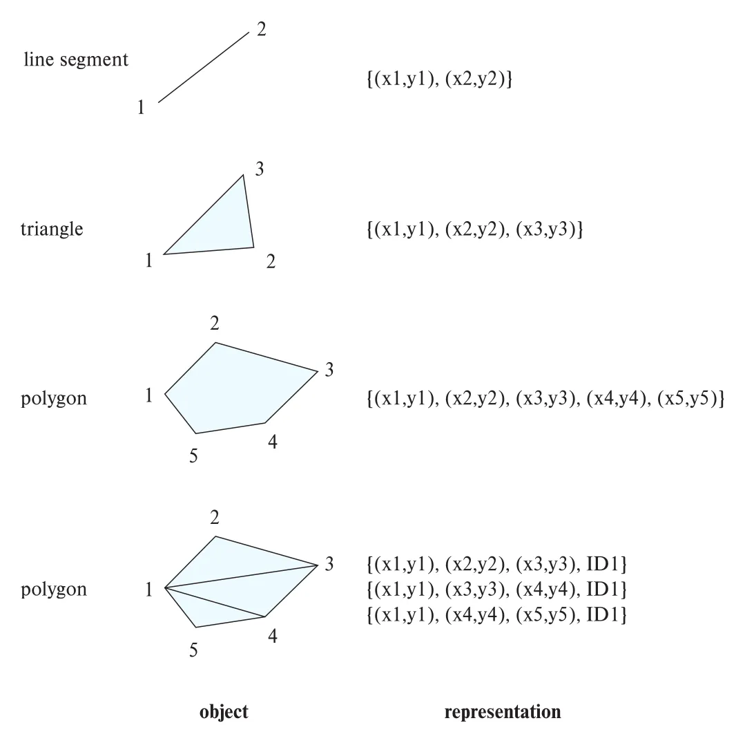 Figure 8.5 · PDF p. 418 · line segment, triangle, polygon의 geometric representation
기본 geometric construct는 다음처럼 표현된다.
| geometric construct | representation |
|---|---|
| point | 2D에서는 (x, y), geographic map에서는 latitude/longitude |
| line segment | 두 endpoint coordinates |
polyline, linestring | connected line segments의 endpoint list |
| polygon | vertices를 순서대로 나열해 boundary 표현 |
| triangulated polygon | polygon을 triangle set으로 나누고 각 triangle에 polygon ID 부여 |
polyline은 road처럼 폭이 map 전체 scale에 비해 작아 line으로 취급해도 되는 feature에 유용하다. Arbitrary curve도 작은 line segment sequence로 근사할 수 있다. 일부 system은 circular arc를 primitive로 지원해 curve를 arc sequence로 표현한다.
Polygon은 vertex list로 boundary를 나타낼 수 있다. 또는 polygon을 triangle set으로 나누는 triangulation을 사용할 수 있다. Triangulation은 모든 polygon에 적용 가능하며, 각 triangle tuple이 원래 polygon의 identifier를 갖게 하면 1NF relational representation에 넣기 쉽다.
List-based representation은 query processing에 편하지만, list 자체가 non-atomic value이므로 NFNF 성격이 있다. Fixed-size tuple과 1NF representation을 유지하려면 polyline ID를 두고 segment마다 별도 tuple을 만들거나, polygon을 triangle tuple들로 분해한다.
3D representation도 2D와 비슷하다. Point에는 z component가 추가되고, triangle/rectangle/polygon 같은 planar figure는 3D coordinates를 갖는다. Polyhedron은 tetrahedron으로 분해하거나, faces를 polygon으로 나열하고 각 face의 inside 방향을 표시해 표현할 수 있다.
PostGIS와 SQL Server는 geometry와 geography type을 지원하며, 그 subtype으로 point, linestring, curve, polygon, multipoint, multilinestring, multicurve, multipolygon 등을 둔다. OGC textual representation 예는 다음과 같다.
LINESTRING(1 1, 2 3, 4 4)
POLYGON((1 1, 2 3, 4 4, 1 1))ST_GeometryFromText()와 ST_GeographyFromText() 같은 conversion function은 text representation을 internal geometry/geography object로 변환한다. ST_Union()과 ST_Intersection()은 linestring, polygon 같은 geometric objects의 union/intersection을 계산한다. 실제 function name과 syntax는 DBMS마다 다를 수 있다.
Map data에서 road line segments는 단순 objects의 모음이 아니라 graph를 이룬다. 이런 구조를 spatial network 또는 spatial graph라고 한다. Vertex에는 spatial location이 있고, edge에는 distance, lanes, average speed by time of day 같은 nonspatial attribute도 붙을 수 있다.
8.4.2 Design Databases
computer-aided-design(CAD) system은 전통적으로 editing 중에는 design data를 memory에 두고, session 끝에 file로 저장했다. 이 방식은 몇 가지 문제가 있다.
| 문제 | 설명 |
|---|---|
| 변환 비용 | memory representation과 file representation 사이 변환 code/time cost 발생 |
| 부분 접근 어려움 | 일부만 필요해도 전체 file을 읽어야 할 수 있음 |
| 대형 design 한계 | 대형 integrated circuit, airplane design은 전체를 memory에 올리기 어려움 |
Object-oriented database가 CAD 요구에서 동기를 얻은 이유도 여기에 있다. Design의 component를 object로 표현하고, object 사이 connection으로 design structure를 나타내면 database가 partial retrieval, object identity, relationship traversal을 지원할 수 있다.
Design database의 objects는 보통 geometric objects다. 2D에서는 point, line, triangle, rectangle, polygon이 기본이고, 3D에서는 sphere, cylinder, cuboid 같은 object를 union/intersection/difference로 조합한다.
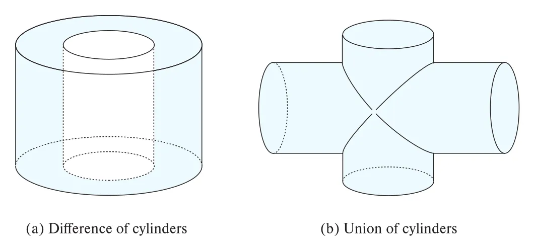 Figure 8.6 · PDF p. 420 · cylinder difference와 union으로 만든 complex 3D objects
Figure 8.6은 complex 3D object가 simpler objects의 set operation으로 만들어질 수 있음을 보여준다. 3D surface는 wireframe model로도 표현할 수 있는데, 이는 surface를 line segments, triangles, rectangles 같은 simpler objects의 집합으로 모델링하는 방식이다.
Design database에는 material 같은 nonspatial information도 저장된다. 이런 attribute는 일반 data modeling으로 처리할 수 있지만, spatial aspect에는 spatial query와 spatial integrity constraint가 필요하다. 예를 들어 “two pipes should not be in the same location” 같은 constraint는 설계 오류를 사전에 잡기 위해 중요하다. 이런 check를 효율적으로 하려면 multidimensional spatial index가 필요하다.
8.4.3 Geographic Data
Geographic data는 spatial data이지만 CAD design data와 성격이 다르다. Map과 satellite image가 대표적이다. Geographic database는 boundary, river, road 같은 location information뿐 아니라 elevation, soil type, land usage, annual rainfall 같은 location-associated information도 저장한다.
8.4.3.1 Applications of Geographic Data
Geographic database의 application은 매우 넓다.
| application | 예 |
|---|---|
| online map/navigation | route search, nearby place search |
| public utility network | telephone, electric-power, water-supply cable/pipe maps |
| land-use/ecology/planning | land usage, ecological planning |
| land records | ownership boundary tracking |
Public utility에서는 buried cable/pipe location이 특히 중요하다. 정확한 map이 없으면 한 utility의 공사가 다른 utility의 pipe/cable을 손상시켜 대규모 service disruption을 만들 수 있다. GPS 같은 accurate location-finding system과 geographic database를 결합하면 이런 위험을 줄일 수 있다.
8.4.3.2 Representation of Geographic Data
Geographic data representation은 크게 raster data와 vector data로 나뉜다.
| 표현 | 구조 | 장점 | 한계/적합하지 않은 경우 |
|---|---|---|---|
raster data | bitmap/pixel map, tile, grid/array | satellite image, temperature grid처럼 본질적으로 grid인 data에 적합 | road boundary처럼 정밀 geometry는 pixel resolution에 좌우됨 |
vector data | point, line segment, polyline, polygon, polyhedron | road, lake, boundary, country polygon처럼 shape가 중요한 data에 정확/compact | satellite image처럼 본질적으로 raster인 data에는 부적합 |
Raster data는 2D 또는 그 이상 차원의 pixel map이다. Satellite image는 대표적인 2D raster data다. Image 자체뿐 아니라 corner latitude/longitude, resolution, pixel당 area 정보가 함께 필요하다. Raster data는 보통 fixed-size area를 덮는 tiles로 나누어 저장한다. User interface가 zoom level을 정하면 해당 zoom level에서 화면 영역과 overlap하는 tiles만 가져와 표시한다.
Raster는 3D/temporal dimension도 가질 수 있다. 예를 들어 지역별 고도별 temperature, 시간별 surface temperature measurement는 3D 또는 time dimension이 추가된 array로 볼 수 있다.
Vector data는 geometric primitives로 만든다. Road는 polyline, lake나 state/country boundary는 complex polygon으로 표현된다. River처럼 폭이 중요한 경우에는 polygon으로, 폭을 무시해도 되는 경우에는 curve/polyline으로 표현할 수 있다.
Topographical information은 raster로 표현할 수도 있고 vector로 표현할 수도 있다. Raster라면 surface point마다 elevation을 grid로 저장한다. Vector라면 elevation이 거의 같은 region을 polygon으로 나누거나, surface를 triangle로 나누고 각 vertex의 latitude/longitude/elevation을 저장한다. 후자를 triangulated irregular network(TIN)라고 하며, 3D view 생성에 유용한 compact representation이다.
GIS는 보통 raster와 vector data를 모두 포함하고, display에서 여러 layer를 merge한다. 예를 들어 satellite image 위에 road, building, landmark vector data를 overlay해 hybrid map을 만든다. Map은 여러 layer를 bottom-to-top order로 표시하며, higher layer가 lower layer 위에 보인다.
흥미롭게도 vector로 저장된 data도 browser로 보낼 때는 raster로 변환될 수 있다. JavaScript가 비활성화된 browser에서도 map을 표시할 수 있고, end user가 vector data를 직접 추출해 쓰는 것을 막을 수 있기 때문이다.
8.4.4 Spatial Queries
Spatial query는 location과 geometry 관계를 조건으로 삼는다. 대표 유형은 다음과 같다.
| query type | 의미 | 예 |
|---|---|---|
region query | 지정 region 안에 부분/전체가 들어가는 object 검색 | 특정 town boundary 안의 retail shops 찾기 |
nearness query | 특정 location 근처의 object 검색 | 특정 point 주변 restaurants 찾기 |
nearest-neighbor query | 지정 point와 가장 가까운 object 검색 | 가장 가까운 gasoline station 찾기 |
spatial graph query | road/train network 같은 spatial graph 위의 query | 두 location 사이 shortest path |
spatial join | 두 spatial relation의 object들이 intersect/contain/overlap하는 쌍 또는 intersection region 계산 | rainfall region과 population density region overlap |
PostGIS는 ST_Contains(), ST_Overlaps(), ST_Disjoint(), ST_Touches() 같은 predicates를 제공한다. 예를 들어 shop relation에 location attribute가 point type이고, query region이 polygon이라면 ST_Contains(region, location)으로 region 안의 shop을 찾을 수 있다.
Nearness query는 distance가 중요하다. ST_Distance()는 두 geometry/geography object 사이 minimum distance를 계산할 수 있고, distance threshold 안의 objects를 찾거나 minimum distance를 가진 nearest neighbor를 찾는 데 사용된다.
Spatial graph query는 navigation system과 직접 연결된다. Road network나 train network를 spatial graph로 표현하면, 두 위치 사이 shortest path, fastest path, constrained route를 찾을 수 있다.
Spatial query는 보통 spatial condition과 nonspatial condition을 함께 가진다. 예를 들어 “채식 메뉴가 있고 한 끼 가격이 $10 미만인 가장 가까운 restaurant”은 distance condition, menu attribute, price attribute를 함께 평가해야 한다.
8.5 Summary
Chapter 8의 핵심은 relational model의 atomic/fixed-schema 가정이 현대 application에서 확장되어야 하는 지점을 보여주는 것이다. Semi-structured data는 schema flexibility와 nested value를 제공하고, JSON/XML은 application/data exchange의 실용적 representation이다. RDF/knowledge graph는 web-scale fact와 relationship을 graph로 다루며, SPARQL은 triple pattern 기반 query를 제공한다.
Object orientation은 database type system을 richer하게 만들거나, application object와 relational database 사이 mapping을 자동화한다. Textual data는 schema가 아니라 keyword/relevance 중심으로 검색되고, TF-IDF/PageRank/precision/recall 같은 IR 개념이 필요하다. Spatial data는 geometry/geography type, raster/vector representation, spatial query와 spatial index를 요구한다.
연결 관계
Chapter 7의 1NF/atomic domain 논의가 Chapter 8의 출발점이다. Chapter 7은 atomic value를 가정해야 FD/normal form 이론을 깔끔하게 전개할 수 있음을 보여줬고, Chapter 8은 그 가정이 application 현실에서는 언제 부담이 되는지를 보여준다.
Chapter 6의 E-R model도 계속 연결된다. Composite attribute, multivalued attribute, specialization/generalization, aggregation은 JSON/XML nested data, object-relational inheritance, RDF reification과 구조적으로 닮아 있다.
Chapter 9에서는 web service, application architecture, data-access layer, ORM이 더 직접적으로 이어진다. Chapter 14/15에서는 spatial query processing과 spatial indexing이 더 깊게 다뤄진다. Chapter 24/29/30/31 쪽은 object/complex data/XML/information retrieval의 심화 방향이다.
오해하기 쉬운 내용
| 오해 | 정리 |
|---|---|
| Complex data type은 relational model을 대체한다 | 많은 경우 relational DB 위에 JSON/XML/object/spatial extension이 붙는 식으로 공존한다 |
| JSON은 항상 normalized schema보다 낫다 | Join 없이 object 단위 접근이 빠를 수 있지만 verbose하고 parsing/storage cost가 크다 |
| XML과 JSON은 같은 용도라 완전히 대체 가능하다 | 둘 다 nested text representation이지만 XML은 tag/document exchange 전통이 강하고 JSON은 web API/object exchange에 특히 강하다 |
| RDF graph는 일반 graph DB와 완전히 같다 | RDF는 subject-predicate-object triple 기반 representation이며, graph interpretation이 자연스러운 것이다 |
| ORM을 쓰면 SQL을 몰라도 된다 | ORM은 SQL을 숨기지만, 성능 문제와 complex query에서는 SQL/relational model 이해가 필요하다 |
| PageRank가 query relevance 그 자체다 | PageRank는 query-independent popularity score이고 TF-IDF 등 content relevance와 결합된다 |
| Precision과 recall은 항상 동시에 높일 수 있다 | 보통 더 많이 retrieve하면 recall은 오르지만 precision은 떨어질 수 있다 |
| Spatial data는 좌표만 저장하면 된다 | geometry/geography type, raster/vector choice, spatial predicate, index, integrity constraint가 함께 필요하다 |
면접 질문
- Relational model의
atomic value가정이 modern application에서 왜 문제가 될 수 있는지 설명하라. wide column,sparse column,multivalued data type,nested data type의 차이를 설명하라.- JSON이 web service와 mobile/browser application에서 널리 쓰이는 이유와 단점을 말하라.
- XML의 tag/nesting 구조가 organization-to-organization data exchange에 왜 유용한지 설명하라.
- RDF triple의
subject,predicate,object를 설명하고, RDF가 E-R model과 어떻게 다른지 말하라. - SPARQL의 triple pattern과 shared variable이 join처럼 동작하는 방식을 예로 설명하라.
- Object-relational DBMS, ORM, OODB의 차이와 trade-off를 설명하라.
reference type과 path expression이 join을 어떻게 숨기는지 설명하라.TF-IDF에서 TF와 IDF가 각각 어떤 문제를 해결하는지 설명하라.PageRank가 hyperlink graph를 이용해 page importance를 계산하는 직관을 설명하라.precision,recall,precision@K의 차이를 설명하라.raster data와vector data의 차이를 spatial/geographic data 예로 설명하라.region query,nearness query,nearest-neighbor query,spatial join의 차이를 설명하라.