개요
query optimization은 하나의 query를 처리할 수 있는 여러 query-evaluation plan 중 estimated cost가 가장 낮거나 충분히 낮은 plan을 고르는 과정이다. 사용자는 SQL을 사람이 이해하기 쉽게 작성할 뿐, efficient execution을 암시하도록 query를 쓸 책임이 없다. DBMS는 같은 의미의 여러 relational-algebra expressions와 여러 physical algorithms/access paths를 비교해 실행 전략을 구성해야 한다.
Chapter 15가 selection, sorting, join, aggregation, pipelining 같은 physical operators와 cost model을 다루었다면, Chapter 16은 그 재료들을 조합해 어떤 plan을 선택할지 다룬다. 핵심은 두 층이다. 첫째, relational-algebra level에서 더 싼 equivalent expression으로 바꾼다. 둘째, 각 operation에 사용할 algorithm, index, materialization/pipelining 방식을 선택한다.
핵심 개념
query optimizer는 equivalent relational expressions를 만들고, 이를 physicalquery-evaluation plan으로 annotate한 뒤, statistics와 cost estimates로 plan을 비교한다.equivalence rule은 두 relational-algebra expression이 모든 legal database instance에서 같은 결과를 낸다는 사실을 이용해 expression을 변환하는 규칙이다.logical equivalence만으로 충분하지 않다. 같은 expression도 hash join, merge join, indexed nested-loop join, pipelining/materialization 선택에 따라 plan cost가 크게 달라진다.- Cost difference는 several orders of magnitude까지 벌어질 수 있으므로, 복잡한 query는 optimizer가 plan 선택에 상당한 시간을 쓰는 것이 합리적이다.
- Optimizer의 기본 흐름은
equivalent expression generation -> physical plan annotation -> statistics/cost estimation -> plan choice다. explain또는 GUI plan viewer는 DBMS가 선택한 evaluation plan과 optimizer cost를 보여준다. 단 cost unit은 seconds나 I/O count가 아니라 DBMS 내부 cost model 단위일 수 있다.
세부 정리
16.1 Overview
Query optimization은 “같은 결과를 내면서 더 싸게 계산하는 plan”을 찾는 문제다. 예를 들어 “Music department instructors의 이름과 그들이 가르치는 course title을 찾아라”라는 query를 생각하자. 처음 relational-algebra expression은 큰 join을 먼저 만들고 나중에 dept_name = "Music" selection을 적용할 수 있다.
이 방식은 instructor ⋈ teaches ⋈ course projection이라는 큰 intermediate relation을 만들 수 있다. 하지만 최종적으로 필요한 것은 Music department instructors에 관한 tuple뿐이다. Selection을 instructor에 먼저 적용하면 intermediate result 크기를 크게 줄일 수 있다.
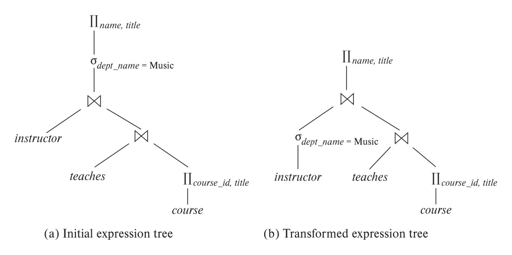 Figure 16.1 · PDF p. 773 · selection pushdown으로 큰 intermediate result를 줄이는 equivalent expression 변환
Figure 16.1의 핵심은 selection을 join 뒤에 할 필요가 없다는 점이다. Query result는 같지만, 먼저 filtering하면 이후 join이 다루는 tuple 수가 줄어든다. 이처럼 relational-algebra expression 변환은 optimizer의 logical optimization 단계다.
하지만 expression만 골라서는 plan이 완성되지 않는다. evaluation plan은 각 operation을 어떤 algorithm으로 실행할지, 어떤 index를 사용할지, edges를 pipelined로 둘지 materialized로 둘지까지 정의한다. Figure 16.2는 Figure 16.1(b)의 transformed expression에 대해 selection은 index를 쓰고, 한 join은 hash join, 다른 join은 sort 후 merge join을 쓰는 physical plan 예시다.
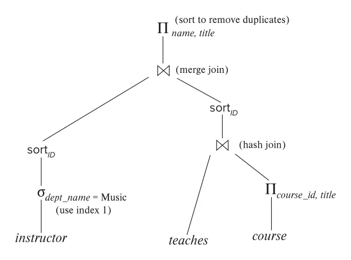 Figure 16.2 · PDF p. 774 · index selection, hash join, sort/merge join, pipelining을 포함한 query-evaluation plan
Figure 16.2에서 edges는 별도 표시가 없으면 pipelined라고 가정한다. pipelined edge는 producer output이 disk temporary relation으로 쓰이지 않고 consumer로 직접 전달되는 edge다. materialized edge는 output을 disk에 쓰고 consumer가 다시 읽는 edge다. Figure 16.2에는 materialized edge가 없지만, sort나 hash join 같은 operator 내부는 Chapter 15에서 본 것처럼 suboperators와 internal materialization을 가질 수 있다.
Optimizer가 least-cost plan을 찾는 과정은 개념적으로 세 단계다.
| 단계 | 내용 |
|---|---|
| logical alternatives | equivalence rules로 original expression과 같은 결과를 내는 expressions 생성 |
| physical alternatives | 각 expression의 operations에 algorithms, access paths, pipelining/materialization annotations 부여 |
| cost comparison | relation sizes, index depths, distinct values 같은 statistics와 Chapter 15 cost formula로 estimated cost 계산 |
실제 optimizer는 이 세 단계를 완전히 분리하지 않는다. 어떤 expression을 만들고 즉시 physical plan으로 annotate해 cost를 추정한 뒤, 다시 다른 expression을 생성하는 식으로 interleaving한다. 모든 후보를 끝까지 전개하면 search space가 너무 크기 때문이다.
Note 16.1의 explain 기능은 optimizer가 고른 plan을 관찰하는 도구다. PostgreSQL과 MySQL은 explain <query> 계열을 제공하고, Oracle/DB2/SQL Server도 각각 plan을 보는 방법을 제공한다. 다만 plan cost는 보통 seconds 같은 외부 단위가 아니라 optimizer 내부 cost model 단위다. PostgreSQL처럼 “first result를 내는 cost”와 “all results를 내는 cost”를 구분해 보여주는 시스템도 있다.
정리하면 Chapter 16의 optimizer는 다음 자료를 함께 써야 한다.
| 필요한 자료 | 어디서 오는가 | 쓰임 |
|---|---|---|
| equivalence rules | Section 16.2 | logically equivalent expressions 생성 |
| result statistics estimation | Section 16.3 | intermediate result size, distinct values 추정 |
| physical operator cost | Chapter 15 | selection/sort/join/materialization cost 추정 |
| plan enumeration/choice | Section 16.4 | estimated cost가 낮은 evaluation plan 선택 |
| materialized views | Section 16.5 | 미리 계산된 result를 query에 재사용 |
16.2 Transformation of Relational Expressions
같은 query는 여러 relational-algebra expressions로 표현될 수 있고, expression마다 evaluation cost가 다를 수 있다. 두 expressions가 모든 legal database instance에서 같은 set of tuples를 생성하면 equivalent하다고 한다. Tuple order는 상관없다. SQL은 실제로 multiset semantics를 쓰므로 SQL용 equivalence는 같은 multiset을 생성해야 하지만, 이 장의 기본 설명은 set-based relational algebra에 기반한다.
16.2.1 Equivalence Rules
equivalence rule은 두 expression form이 equivalent하다는 규칙이다. Optimizer는 이 규칙을 양방향으로 적용해 logically equivalent expressions를 만든다. 규칙은 correctness를 보장할 뿐, 어느 쪽이 더 싸다는 뜻은 아니다. Cost 판단은 statistics와 physical plan cost estimation으로 따로 해야 한다.
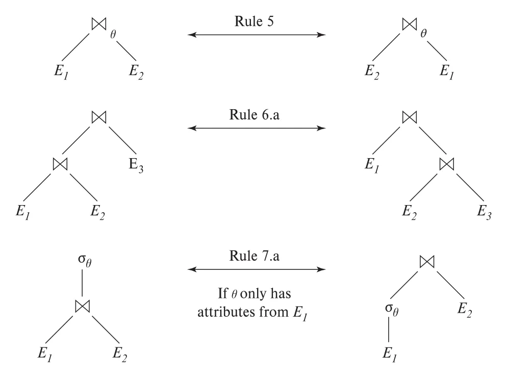 Figure 16.3 · PDF p. 777 · join commutativity/associativity와 selection distribution을 tree로 표현한 equivalence rules
원문 규칙을 optimizer 관점으로 묶으면 다음과 같다.
| 목적 | 원문 rule | 핵심 equivalence | 왜 중요한가 |
|---|---|---|---|
| selection 분해/재배열 | 1, 2 | sigma_theta1 AND theta2(E) ≡ sigma_theta1(sigma_theta2(E)), selections are commutative | predicate를 더 아래로 밀거나 selective한 조건을 먼저 적용할 수 있음 |
| projection 축약 | 3 | cascade of projection에서 final projection만 유지. pi_L1(pi_L2(...pi_Ln(E))) ≡ pi_L1(E) when L1 subset L2 ... | 불필요한 columns를 중간 결과에서 제거 |
| product/join 결합 | 4 | sigma_theta(E1 × E2) ≡ E1 ⋈_theta E2, sigma_theta1(E1 ⋈_theta2 E2) ≡ E1 ⋈_(theta1 AND theta2) E2 | Cartesian product + selection을 join으로 바꿈 |
| join reorder | 5, 6 | theta/natural join commutativity, natural join associativity | join order search의 수학적 기반 |
| selection pushdown | 7 | sigma_theta1(E1 ⋈_theta E2) ≡ sigma_theta1(E1) ⋈_theta E2 if theta1 only uses attributes of E1 | intermediate relation cardinality를 줄임 |
| projection pushdown | 8 | join에 필요한 attributes와 final output attributes만 남기도록 projection을 아래로 이동 | intermediate tuple width를 줄임 |
| set operation reorder | 9, 10 | union/intersection commutativity and associativity | set operation evaluation order 선택 |
| selection over set ops | 11 | selection distributes over union/intersection/set difference | set operation 전에 filtering 가능 |
| projection over union | 12 | pi_L(E1 union E2) ≡ pi_L(E1) union pi_L(E2) when schemas match | union 전에 columns 축소 |
| aggregation selection pushdown | 13 | sigma_theta(G gamma_A(E)) ≡ G gamma_A(sigma_theta(E)) when theta only uses group-by attributes G | group-by 전에 tuple 수 축소 |
| outer join 변환 | 14-16 | full outer join commutativity, left/right exchange, null rejecting predicate면 outer join -> inner join | outer join을 더 싼 inner join으로 바꿀 기회 |
Selection pushdown과 projection pushdown은 optimizer의 가장 직관적인 변환이다. Selection pushdown은 rows를 줄이고, projection pushdown은 columns를 줄인다. 둘 다 intermediate relation size를 줄여 이후 sort/join/hash/materialization cost를 낮춘다.
Projection pushdown은 조금 조심해야 한다. Join condition에 필요한 attributes는 final output에 없더라도 남겨야 한다. 원문 rule 8.b는 이 점을 formal하게 표현한다. Final output list L1 ∪ L2 외에, join condition theta에 쓰이는 attributes L3, L4를 각 input projection에 포함해야 join 자체를 계산할 수 있다.
Outer join 관련 rule은 inner join보다 훨씬 제한적이다. 예를 들어 sigma_year=2017(instructor ⟕ teaches)에서 selection을 단순히 teaches 아래로 밀면, course를 전혀 가르치지 않은 instructor tuple이 left outer join 결과에 null-extended tuple로 살아남을 수 있어 결과가 달라진다. 반면 year=2017 같은 predicate는 teaches 쪽 attribute가 null이면 unknown이 되어 tuple을 제거하므로, 전체 selection이 outer join의 null-extended tuples를 제거하는 경우에는 left outer join을 inner join으로 바꿀 수 있다. 이런 predicate를 null rejecting predicate라고 한다.
또 다른 주의점은 outer join associativity다. Inner/natural join은 associativity가 성립하지만, outer join은 일반적으로 성립하지 않는다. 원문 예시처럼 (r ⟕ s) ⟕ t와 r ⟕ (s ⟕ t)는 null이 붙는 위치가 달라져 서로 다른 결과를 낼 수 있다.
16.2.2 Examples of Transformations
Section 16.1의 Music department query는 rule 7.a, 즉 selection pushdown의 예다. 처음에는 큰 join 후 dept_name = "Music"을 적용했지만, selection predicate가 instructor attributes만 사용하므로 selection을 instructor 아래로 내릴 수 있다.
더 복잡한 예로 dept_name = "Music" AND year = 2017을 함께 요구하면, predicate가 instructor와 teaches 양쪽 attributes를 포함한다. 이 경우 먼저 join associativity(rule 6.a)로 (instructor ⋈ teaches) ⋈ course_projection 형태를 만들고, selection cascade(rule 1)로 predicate를 dept_name = "Music"과 year = 2017로 분해한 뒤, 각각을 해당 relation 아래로 pushdown(rule 7.a)할 수 있다.
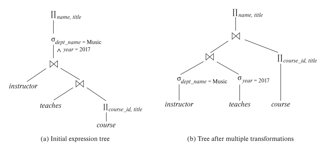 Figure 16.4 · PDF p. 782 · join associativity와 selection cascade/pushdown을 연속 적용한 multiple transformations
이 예시는 equivalence rules 집합이 반드시 minimal하지 않을 수 있음을 보여준다. Rule 7.b는 rule 1과 rule 7.a로 유도될 수 있다. Nonminimal rule set은 같은 equivalent expression을 여러 경로로 생성해 search space를 불필요하게 키우므로, 실제 optimizer는 중복을 줄이기 위해 minimal하거나 잘 통제된 rule set을 선호한다.
Projection pushdown 예도 중요하다. instructor ⋈ teaches의 intermediate schema에는 ID, name, dept_name, salary, course_id, sec_id, semester, year가 들어갈 수 있지만, 이후 필요한 것은 name과 course_id뿐이다. 따라서 join 뒤 또는 join 전후 적절한 위치에 pi_name,course_id를 넣으면 intermediate tuple width가 줄어든다.
16.2.3 Join Ordering
Join order는 query cost를 크게 좌우한다. Natural join은 associative이고 commutative이므로, 같은 relations를 다양한 순서로 join해도 같은 logical result를 얻을 수 있다.
하지만 cost는 전혀 다를 수 있다. Music query에서 teaches ⋈ course_projection을 먼저 계산하면 “가르쳐진 모든 course”에 대한 큰 relation이 생긴다. 반대로 sigma_dept_name="Music"(instructor) ⋈ teaches를 먼저 계산하면 Music department instructors가 가르친 courses만 남아 훨씬 작을 가능성이 높다.
나쁜 join order는 Cartesian product를 만들 수도 있다. 예를 들어 instructor ⋈ course_projection은 common attribute가 없다면 사실상 Cartesian product가 되어 a * b tuples를 만들 수 있다. Optimizer는 join commutativity/associativity를 이용해 이런 order를 피하고, join predicates가 있는 relations를 먼저 결합하도록 plan을 바꿀 수 있다.
16.2.4 Enumeration of Equivalent Expressions
Optimizer는 equivalence rules로 equivalent expressions를 체계적으로 생성할 수 있다. 개념적 procedure는 Figure 16.5와 같다. 집합 EQ를 original expression E로 시작하고, EQ 안의 각 expression과 각 equivalence rule을 match한다. 어떤 subexpression이 rule의 한쪽 form과 match하면, 그 subexpression을 rule의 다른쪽 form으로 바꾼 새 expression을 만들고 EQ에 추가한다. 새 expression이 더 이상 생성되지 않을 때 멈춘다.
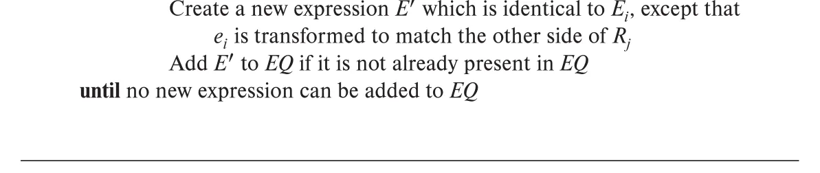 Figure 16.5 · PDF p. 785 · equivalence rules를 반복 적용해 equivalent expressions 집합을 생성하는 procedure
이 naive enumeration은 time과 space 모두 매우 비싸다. Optimizer는 두 가지 아이디어로 비용을 줄인다.
| 최적화 | 의미 |
|---|---|
| shared subexpressions | 새 expression은 기존 expression과 대부분 subtrees를 공유하므로, representation이 같은 subexpression을 공유하게 만든다 |
| cost-aware pruning | 모든 equivalent expression을 만들지 않고, cost estimate를 이용해 비싼 후보나 불필요한 후보를 배제한다 |
일부 optimizer는 equivalence rules를 heuristic하게 적용한다. 예를 들어 “selection을 아래로 밀어라”, “projection을 아래로 밀어라” 같은 rule을 cost가 줄어드는 방향으로 반복 적용한다. 이 방식은 빠르지만 optimal plan을 보장하지 않는다. 반대로 cost-based optimizer는 Section 16.4에서 보듯 후보 plan cost를 계산해 더 체계적으로 선택하지만, search space 관리가 핵심 문제가 된다.
16.3 Estimating Statistics of Expression Results
query optimizer가 계획을 고르려면 각 연산자의 입력 크기와 출력 크기를 추정해야 한다. selection, join, aggregation 같은 연산은 결과 tuple 수와 block 수에 따라 비용이 크게 달라지므로, optimizer는 식 트리의 아래에서 위로 올라가며 각 subexpression의 statistics를 추정한다. 이 추정은 정확한 값이 아니라 근사치지만, 좋은 계획과 나쁜 계획의 차이가 보통 매우 크기 때문에 충분히 유용하다.
16.3.1 Catalog Information
DBMS는 system catalog에 relation, index, attribute에 대한 통계를 저장한다. 대표적인 값은 다음과 같다.
| 표기 | 의미 |
|---|---|
nr | relation r의 tuple 수 |
br | relation r가 차지하는 block 수 |
lr | relation r의 tuple 하나의 byte 크기 |
fr | block 하나에 들어가는 r의 tuple 수, 즉 blocking factor |
V(A, r) | relation r에서 attribute A가 갖는 distinct value 수 |
V(𝒜, r) | attribute 집합 𝒜의 distinct tuple 수 |
고정 길이 record라면 대략 다음 관계를 쓴다.
A가 r의 key이면 모든 tuple이 다른 A 값을 가지므로 V(A, r) = nr이다. index에 대해서는 B+-tree의 height, leaf page 수, key distinct value 같은 통계가 중요하다.
통계는 매 update마다 즉시 갱신하지 않는다. 그렇게 하면 통계 유지 자체가 비싸진다. 보통 DBMS는 부하가 낮을 때 전체 relation을 scan하거나, 큰 relation은 sampling으로 추정하고, 사용자가 analyze, runstats 같은 명령으로 갱신을 요청할 수 있게 한다. 실행 중 실제 cardinality가 optimizer 추정과 크게 다르면 통계 갱신을 trigger할 수도 있다.
histogram은 값 분포가 균등하지 않을 때 중요한 통계다. equi-width histogram은 value range를 같은 폭으로 나누고, equi-depth histogram은 각 bucket에 들어가는 tuple 수가 비슷해지도록 나눈다. query optimization에는 skew를 더 잘 잡는 equi-depth histogram이 더 유리한 경우가 많다. bucket별 distinct value 수나 most frequent values를 같이 저장하면 equality selection과 range selection의 추정이 더 좋아진다.
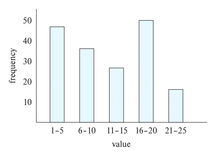 Figure 16.6 · PDF p. 788 · attribute 값 분포를 bucket으로 요약한 histogram 예시
16.3.2 Selection Size Estimation
σA=a(r) 같은 equality selection의 기본 추정은 균등 분포를 가정한 nr / V(A, r)이다. 단, histogram이나 most frequent values에 a의 실제 빈도가 있으면 그 값을 사용한다. 예를 들어 특정 학과나 특정 연도가 유난히 많다면 단순 균등 가정은 크게 빗나갈 수 있다.
σA<=v(r) 같은 comparison selection은 min(A, r), max(A, r)가 있을 때 다음처럼 추정할 수 있다.
if v < min(A, r):       0
if v >= max(A, r):      nr
otherwise:              nr * (v - min(A, r)) / (max(A, r) - min(A, r))
optimization 시점에 v 값을 알 수 없으면, 흔한 fallback으로 nr / 2를 사용한다. histogram이 있으면 위의 선형 균등 가정보다 bucket별 빈도를 이용해 더 정교하게 추정한다.
복합 predicate는 각 simple condition의 selectivity를 결합해 추정한다. simple condition θi의 결과 tuple 수 추정치를 si라고 하면 si / nr이 selectivity다.
| 조건 형태 | 추정 방식 |
|---|---|
σθ1∧θ2∧...∧θn(r) | independence를 가정하고 nr * (s1/nr) * (s2/nr) * ... * (sn/nr) |
σθ1∨θ2∨...∨θn(r) | inclusion-exclusion의 독립 근사로 nr * (1 - Π(1 - si/nr)) |
σ¬θ(r) | nr - size(σθ(r)) |
SQL의 null 때문에 negation은 조심해야 한다. 비교 결과가 unknown이 될 수 있으므로, 정확도를 높이려면 null value 수나 unknown으로 떨어지는 비율에 대한 통계도 필요하다.
16.3.3 Join Size Estimation
join size estimation은 전체 optimization의 핵심이다. join 순서 하나가 intermediate result 크기를 폭발시킬 수 있기 때문이다.
| 연산/상황 | 결과 크기 추정 |
|---|---|
r × s | nr * ns tuples, tuple size는 대략 lr + ls |
r(R) ⋈ s(S), R ∩ S = ∅ | natural join이 Cartesian product와 같음 |
공통 attribute가 R의 key | 결과 tuple 수는 최대 ns |
공통 attribute가 S의 foreign key이고 R을 참조 | matching parent가 존재한다고 보면 결과는 정확히 ns |
공통 attribute A가 어느 쪽 key도 아님 | 균등 분포 가정으로 nr * ns / V(A, s)와 nr * ns / V(A, r) 중 더 작은 값 |
theta join | σθ(r × s)로 보고 selection 추정 적용 |
예를 들어 student ⋈ takes에서 nstudent = 5000, ntakes = 10000, V(ID, student) = 5000, V(ID, takes) = 2500이라고 하자. takes.ID가 student.ID를 참조하는 foreign key이면 결과는 정확히 10000 tuples다. foreign key 정보를 쓰지 않으면 5000*10000/2500 = 20000과 5000*10000/5000 = 10000 중 작은 10000으로 추정한다.
여러 attribute로 join하면 각 attribute의 selectivity를 결합하거나, histogram을 bucket별로 맞추어 더 정교하게 계산한다. 결국 optimizer가 알고 싶은 것은 “이 join을 지금 수행하면 다음 연산자에게 얼마나 큰 relation을 넘기는가”다.
16.3.4 Size Estimation for Other Operations
다른 relational operation도 cardinality 추정 규칙이 필요하다.
| 연산 | 결과 크기 추정 |
|---|---|
πA(r) | duplicate 제거 후 V(A, r) |
G γA(r) | grouping attribute G 기준 group 수이므로 V(G, r) |
r ∪ s | 일반적인 상한 nr + ns |
r ∩ s | 일반적인 상한 min(nr, ns) |
r - s | 일반적인 상한 nr |
| left outer join | ` |
| right outer join | ` |
| full outer join | ` |
같은 relation에 대한 selection 결과끼리 union, intersection, difference를 수행하는 경우에는 set operation을 or, and, not predicate가 있는 selection으로 다시 써서 selection size estimation을 적용할 수 있다.
16.3.5 Estimation of Number of Distinct Values
상위 연산자의 비용을 추정하려면 tuple 수뿐 아니라 distinct value 수 V(A, r)의 변화도 추정해야 한다.
selection 결과의 distinct value는 predicate가 attribute를 얼마나 제한하는지에 따라 달라진다. θ가 A = 3을 강제하면 V(A, σθ(r)) = 1이다. A가 몇 개의 지정된 값 중 하나라고 강제하면 그 지정 값 수가 distinct value 추정치가 된다. A op v 같은 range predicate라면 selectivity s를 이용해 대략 V(A, r) * s로 잡는다. predicate가 A와 독립적이라고 보면 min(V(A, r), nσθ(r))을 사용한다.
join 결과에서는 attribute가 어느 relation에서 왔는지가 중요하다. A가 전부 r의 attribute이면 min(V(A, r), n_{r⋈s})로 잡고, 전부 s에서 왔으면 대칭적으로 계산한다. A가 양쪽 relation attribute를 섞은 집합이면, 양쪽 distinct value 조합의 가능한 수와 join 결과 cardinality를 함께 제한으로 둔다.
projection은 선택한 attribute 집합의 distinct value 수를 그대로 사용한다. grouping의 distinct value는 group 수가 되고, sum, count, avg 같은 aggregate 결과는 보수적으로 모두 다를 수 있다고 보기도 한다. min, max는 group 수와 원래 attribute distinct value 수 사이의 작은 쪽으로 제한된다.
16.4 Choice of Evaluation Plans
Expression generation만으로는 query optimization이 끝나지 않는다. 같은 logical operation도 nested-loop join, indexed nested-loop join, hash join, sort-merge join, index scan, relation scan처럼 여러 physical algorithm으로 구현될 수 있다. evaluation plan은 각 operation에 어떤 algorithm을 쓸지, operation 사이를 pipelining할지 materialization할지까지 정한 실행 계획이다.
cost-based optimizer는 query와 equivalent한 evaluation plans의 공간을 탐색하고, Section 16.3의 statistics estimate와 Chapter 15의 physical algorithm cost model을 결합해 least estimated cost plan을 선택한다. 다만 search space가 너무 크기 때문에, 실제 optimizer는 dynamic programming, memoization, pruning, heuristic을 함께 쓴다.
16.4.1 Cost-Based Join-Order Selection
SQL query의 가장 흔한 형태는 여러 relations의 join과 selection predicates다. r1 ⋈ r2 ⋈ ... ⋈ rn처럼 join 순서가 지정되지 않은 logical expression은 매우 많은 join order를 가진다. n = 3만 되어도 12가지 join order가 가능하고, 일반적으로는 다음 수만큼 늘어난다.
n = 7이면 665,280가지, n = 10이면 17.6 billion을 넘는다. 모든 join tree를 단순 열거하는 방식은 금방 불가능해진다.
핵심 최적화는 optimal substructure다. 어떤 plan이 {r1, r2, r3}를 먼저 join한 결과를 이후 r4, r5와 join한다면, {r1, r2, r3}를 만드는 내부 plan은 그 subset에 대한 cheapest plan만 남겨도 된다. 더 비싼 내부 plan은 이후에 붙는 join이 같다면 전체 plan도 더 비싸지기 때문이다. 이 아이디어가 dynamic programming algorithm의 기반이다.
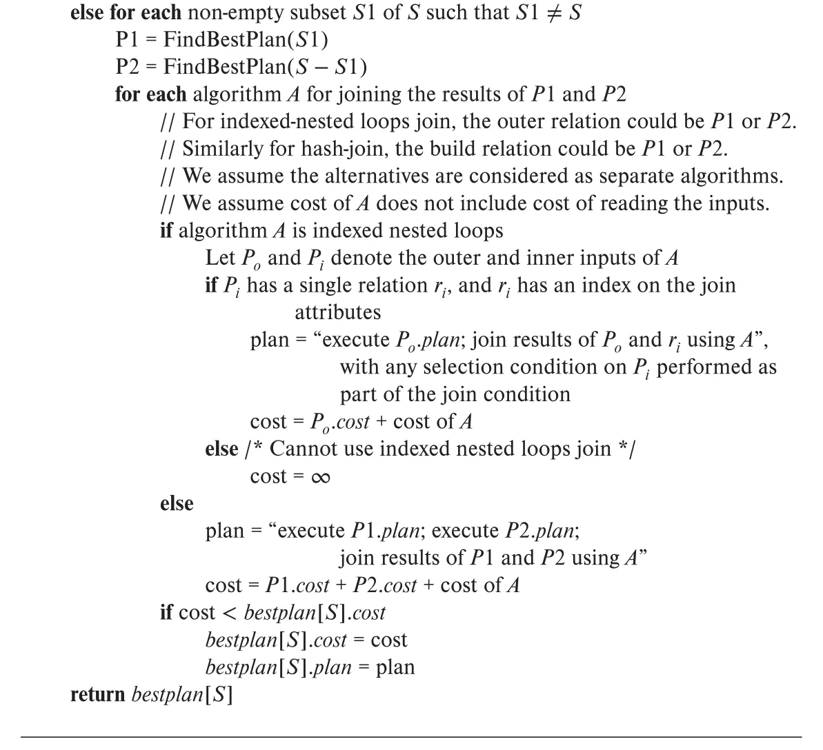 Figure 16.7 · PDF p. 797 · relation subset별 best plan을 저장하며 join order를 찾는 dynamic-programming algorithm
Figure 16.7의 FindBestPlan(S)는 relation set S에 대한 best plan을 associative array bestplan[S]에 저장한다.
| 단계 | 의미 |
|---|---|
이미 계산된 bestplan[S]가 있으면 반환 | 같은 subset을 다시 최적화하지 않는 memoization |
S가 relation 하나이면 access plan 선택 | index scan, relation scan, selection condition 적용 |
S가 여러 relation이면 S1과 S - S1으로 분할 | 가능한 모든 binary join split 탐색 |
각 split마다 P1, P2의 best plan 재사용 | subset plan을 재귀적으로 결합 |
| 가능한 join algorithm을 모두 고려 | indexed nested loops, hash join, sort-merge join 등 |
가장 싼 plan을 bestplan[S]에 저장 | 이후 상위 plan에서 재사용 |
주의할 점은 join cost 계산에서 input read cost를 중복해서 더하지 않는다는 것이다. 이전 operator의 output이 pipelined로 전달된다고 보면, join algorithm cost는 이미 만들어진 input을 읽어오는 비용을 따로 포함하지 않게 조정한다. 단, indexed nested loops join은 inner relation을 별도 scan하지 않고 index lookup을 수행하므로 cost와 plan 구조가 다르게 취급된다.
이 dynamic-programming 방식의 시간 복잡도는 O(3^n)이다. 모든 join order를 열거하는 것보다 훨씬 낫지만, 여전히 relation 수가 커지면 비싸다. 또 merge join처럼 output order가 다음 연산에 도움이 될 수 있으므로, 단순히 subset마다 하나의 best plan만 저장하면 부족하다. 이후 join이나 order by, group by에 유용한 tuple order를 interesting sort order라고 하며, optimizer는 bestplan[S, o]처럼 relation subset S와 interesting sort order o별 best plan을 따로 저장할 수 있다.
Cartesian product를 피하는 것도 중요하다. 두 relation 사이에 join condition이 없는데 먼저 결합하면 큰 intermediate result가 생긴다. 따라서 join graph를 고려해 Cartesian-product-free join order만 생성하도록 search를 줄일 수 있다.
16.4.2 Cost-Based Optimization with Equivalence Rules
Join-order selection은 inner join 중심 query에는 강하지만, aggregation, outer join, set operation, nested query, top-K 같은 연산까지 일반적으로 다루려면 equivalence rules 기반의 general-purpose optimizer가 필요하다.
아이디어는 logical equivalence rules에 physical equivalence rules를 추가하는 것이다. 예를 들어 logical join을 hash join, nested-loops join, sort-merge join 같은 physical operation으로 바꾸는 rule을 추가하면, equivalent expressions 생성 절차가 evaluation plans까지 생성할 수 있다. 이후 각 plan에 cost estimation을 적용해 least-cost plan을 고른다.
하지만 naive rule application은 너무 비싸므로, 실제 구조에는 다음 장치가 필요하다.
| 장치 | 역할 |
|---|---|
| space-efficient expression representation | equivalence rule 적용 때 같은 subexpression을 여러 번 복사하지 않음 |
| duplicate derivation detection | 다른 rule 적용 경로로 같은 expression이 생기는 중복을 제거 |
| memoization 기반 dynamic programming | 같은 subexpression을 다시 최적화하지 않고 memorized optimal plan 반환 |
| pruning | 지금까지 발견한 cheapest plan보다 비싼 후보를 일찍 버림 |
이 계열의 대표적 연구가 Volcano optimizer이며, SQL Server optimizer도 이 접근에 기반한다. 핵심은 “logical equivalence space”와 “physical implementation space”를 한 search framework 안에서 다루되, memoization과 pruning으로 감당 가능한 크기로 유지하는 것이다.
16.4.3 Heuristics in Optimization
Cost-based optimization은 실행 시간을 크게 줄일 수 있지만, optimization 자체도 비용이 든다. 그래서 DBMS는 optimality를 일부 포기하고 optimizer 실행 시간을 줄이는 heuristics를 섞는다.
가장 흔한 heuristic은 다음 둘이다.
| heuristic | 기대 효과 | 주의점 |
|---|---|---|
| perform selections early | tuple 수를 빨리 줄이고 index access 기회를 만듦 | 항상 좋은 것은 아님. 아주 작은 r과 큰 s를 join할 때, s의 selection attribute에는 index가 없고 join attribute에는 index가 있으면 selection pushdown이 오히려 full scan을 유발할 수 있음 |
| perform projections early | temporary relation의 tuple width를 줄임 | join/group/order에 필요한 attributes를 제거하면 안 되고, selection보다 효과가 작을 수 있음 |
System R optimizer는 모든 join tree를 보지 않고 left-deep join order를 중심으로 탐색했다. Left-deep join tree는 각 join의 right operand가 원래 base relation 중 하나인 형태다. 이 구조는 right input이 stored relation이어서 한쪽 input만 pipelined로 흐르게 만들기 쉽고, 따라서 pipelined evaluation에 편리하다.
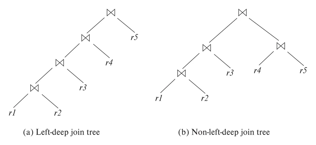 Figure 16.8 · PDF p. 802 · left-deep join tree와 non-left-deep join tree의 구조 차이
Left-deep join order만 보면 가능한 순서는 O(n!)이고, dynamic programming을 결합한 System R 방식은 O(n2^n) 시간에 best left-deep order를 찾을 수 있다. 이는 모든 bushy join tree를 고려하는 O(3^n)보다 작다.
다른 heuristic 방식은 시작 relation을 하나씩 바꿔 n개의 left-deep plan을 만들고, 각 단계에서 “다음에 붙일 best relation”을 access path ranking으로 고르는 식이다. nested-loop join에 inner index가 있는지, sort-merge join이 필요한지 같은 기준으로 후보를 평가한다. 이런 방식은 빠르지만 global optimum을 보장하지 않는다.
실용 optimizer는 보통 optimization cost budget도 둔다. 탐색 예산이 끝나면 그 시점까지 찾은 best plan을 반환한다. 싼 plan을 빨리 찾으면 예산을 줄이고, 현재 best plan이 여전히 비싸면 더 탐색할 가치가 있으므로 예산을 늘릴 수 있다. 또한 같은 query를 constants만 바꿔 반복 실행하는 application을 위해 plan caching을 사용한다. 처음 생성한 query plan을 저장했다가 새 parameter 값에 재사용하는 방식이다. 새 값에 대한 optimal plan이 다를 수 있다는 위험은 있지만, 반복 query에서는 optimization overhead를 크게 줄인다.
16.4.4 Optimizing Nested Subqueries
SQL의 nested subquery는 개념적으로 outer query의 값을 parameter로 받는 함수처럼 볼 수 있다. 예를 들어 다음 query는 각 instructor.ID에 대해 2019년에 가르친 teaches tuple이 존재하는지 검사한다.
select name
from instructor
where exists (
  select *
  from teaches
  where instructor.ID = teaches.ID
    and teaches.year = 2019
);
Subquery가 outer query tuple마다 별도로 실행되는 방식을 correlated evaluation이라고 한다. 이 방식은 outer tuple 수만큼 subquery를 호출하므로 random disk I/O가 많아질 수 있다. Optimizer는 가능하면 nested subquery를 join, semijoin, anti-semijoin으로 바꾸려 한다.
단순 join으로 바꾸면 SQL의 multiset semantics가 깨질 수 있다. 2019년에 여러 section을 가르친 instructor는 join 결과에서 여러 번 나타날 수 있지만, 원래 exists query에서는 존재 여부만 보므로 instructor tuple의 duplicate count가 증가하면 안 된다. 이를 해결하는 연산자가 semijoin이다.
r ⋉θ s의 multiset semijoin은 r의 tuple ri가 r에 n번 등장하고, s에 θ를 만족하는 matching tuple이 하나 이상 있으면 결과에 ri를 그대로 n번 남긴다. matching tuple이 없으면 제거한다. 즉, 오른쪽 relation은 filtering 조건으로만 쓰고, 왼쪽 tuple의 multiplicity를 늘리지 않는다.
위 exists query는 다음처럼 semijoin으로 표현할 수 있다.
in clause도 같은 semijoin 형태로 바꿀 수 있다. 반대로 not exists는 anti-semijoin 또는 anti-join이 맞다. r의 tuple이 s에서 matching tuple을 갖지 않을 때만 결과에 남긴다.
Nested query를 join, semijoin, anti-semijoin이 있는 query로 바꾸는 과정을 decorrelation이라고 한다. Decorrelation이 성공하면 efficient join algorithms를 사용할 수 있어 correlated evaluation보다 훨씬 빠를 수 있다.
Aggregation이 들어간 scalar subquery는 더 어렵다. 예를 들어 “2019년에 1개 초과 section을 가르친 instructor”를 찾는 query는 subquery 내부의 count(*)가 outer instructor.ID마다 따로 계산된다. Decorrelation하려면 teaches를 ID로 group by해서 count(*) as cnt를 만들고, instructor.ID = TID AND 1 < cnt 조건의 semijoin으로 바꾸어야 한다.
모든 nested subquery가 decorrelate될 수 있는 것은 아니다. Scalar subquery는 결과가 하나여야 하며, 여러 tuple을 반환하면 runtime exception이 날 수 있는데, 단순 decorrelated query는 이런 예외 semantics를 그대로 표현하기 어렵다. 따라서 decorrelation 여부도 원칙적으로 cost-based로 판단해야 하고, 많은 optimizer는 복잡한 nested subquery에 대해 제한적인 decorrelation만 수행한다.
16.5 Materialized Views
일반 view는 view definition query만 저장하고, 사용할 때마다 query를 실행해 내용을 계산한다. 반면 materialized view는 view의 contents를 미리 계산해 저장한다. 이는 원래 database contents에서 유도 가능한 redundant data지만, 자주 쓰는 expensive query 결과를 바로 읽을 수 있으므로 query processing을 크게 빠르게 할 수 있다.
예를 들어 학과별 총 급여를 구하는 view가 있다고 하자.
create view department_total_salary(dept_name, total_salary) as
select dept_name, sum(salary)
from instructor
group by dept_name;
이 값을 자주 조회한다면 매번 instructor를 읽고 sum(salary)를 계산하는 대신, materialized view의 tuple 하나를 lookup하는 편이 훨씬 싸다. 특히 sales fact table처럼 수천만 tuple을 aggregate하는 workload에서는 차이가 매우 크다.
16.5.1 View Maintenance
Materialized view의 대가는 최신성 유지다. Base relation이 바뀌면 materialized view도 함께 바뀌어야 한다. 이 작업을 view maintenance라고 한다.
| 방식 | 의미 | trade-off |
|---|---|---|
| manual maintenance | update code마다 view 갱신 로직을 직접 작성 | 빠질 가능성이 높아 error prone |
| trigger-based maintenance | insert/delete/update trigger로 view 갱신 | 자동화 가능하지만 단순 재계산은 비쌈 |
| recomputation | update마다 view 전체를 다시 계산 | 구현은 단순하지만 큰 view에는 비효율적 |
| incremental view maintenance | 변경된 부분만 반영 | 보통 가장 실용적이며 DBMS가 직접 지원 |
| immediate view maintenance | update transaction 안에서 즉시 갱신 | view가 base relation과 일관적이지만 update cost 증가 |
| deferred view maintenance | 나중에 모아서 갱신 | update transaction 부담은 줄지만 view가 일시적으로 stale할 수 있음 |
16.5.2 Incremental View Maintenance
incremental view maintenance는 update를 전체 재계산으로 처리하지 않고, base relation의 변화분만 view에 반영한다. Update는 delete 후 insert로 볼 수 있으므로, 핵심 변화는 insertion set과 deletion set이다. 이런 변화분을 relation 또는 expression의 differential이라고 한다.
16.5.2.1 Join Operation
Materialized view v = r ⋈ s에서 r에 tuple 집합 ir가 insert되었다고 하자. 새 relation은 rnew = rold ∪ ir이고, 새 view는 다음처럼 쓸 수 있다.
즉, view 전체를 다시 만들 필요 없이 ir ⋈ s만 계산해 기존 materialized view에 추가하면 된다. 삭제 dr는 대칭적으로 처리한다.
s에 대한 insert/delete도 같은 방식으로 처리한다.
16.5.2.2 Selection and Projection Operations
Selection view v = σθ(r)는 변화분에도 같은 selection을 적용하면 된다.
Projection view v = πA(r)는 더 조심해야 한다. r(A, B)에 (a, 2), (a, 3)이 있으면 πA(r)에는 (a) 하나만 있다. (a, 2)를 삭제했다고 (a)를 view에서 지우면 안 된다. (a, 3)이 아직 같은 projection result를 지탱하기 때문이다.
해결책은 projection result tuple마다 derivation count를 저장하는 것이다. 삭제 시 t.A의 count를 1 줄이고, count가 0이 되면 tuple을 삭제한다. Insert 시 이미 있으면 count를 1 늘리고, 없으면 count 1로 새 tuple을 넣는다.
16.5.2.3 Aggregation Operations
Aggregation view maintenance도 projection처럼 추가 state가 필요하다.
| aggregate | incremental maintenance 핵심 |
|---|---|
count | group t.G의 count를 insert 시 +1, delete 시 -1, 0이면 group tuple 삭제 |
sum | group sum에 t.B를 더하거나 빼고, count도 함께 유지 |
avg | average를 직접 갱신하지 않고 sum과 count를 유지한 뒤 sum / count로 계산 |
min, max | insert는 비교로 쉽게 처리하지만, 현재 min/max tuple이 delete되면 같은 group의 다른 tuple에서 새 min/max를 찾아야 함 |
sum에서도 count가 필요하다. group sum이 0인 상태와 group에 tuple이 하나도 남지 않은 상태를 구분해야 하기 때문이다. min, max 삭제 처리를 빠르게 하려면 (G, B)에 ordered index를 두면 group별 새 minimum/maximum을 효율적으로 찾을 수 있다.
16.5.2.4 Other Operations
Set operation과 outer join도 incremental maintenance가 가능하다. v = r ∩ s에서 r에 tuple이 insert되면 s에 존재하는지 확인한 뒤 view에 추가한다. 삭제되면 intersection에 있던 tuple을 제거한다. union, set difference도 유사하게 처리하지만 duplicate/multiplicity와 derivation count를 고려해야 한다.
Outer join은 일반 join보다 추가 처리가 필요하다. 예를 들어 r에서 삭제가 일어나면, 이제 r과 match하지 않게 된 s tuple이 null-extended tuple로 나타나야 할 수 있다. Insert는 반대로 기존 null-extended tuple이 실제 match tuple로 대체될 수 있다.
16.5.2.5 Handling Expressions
전체 expression은 작은 subexpression부터 differential을 전파한다. 예를 들어 materialized view가 E1 ⋈ E2이고, base relation r의 insert가 E1에만 영향을 주며 그 변화분이 D1이라면, 최종 join view에 추가할 변화분은 D1 ⋈ E2다. 즉, operation별 differential rule을 expression tree 위로 조립해 전체 materialized view change를 계산한다.
16.5.3 Query Optimization and Materialized Views
Materialized view는 regular relation처럼 optimization 대상이 될 수 있지만, 그 이상으로 query rewrite 기회를 제공한다.
| rewrite 방향 | 예 | optimizer가 따져야 하는 점 |
|---|---|---|
| query를 materialized view로 대체 | r ⋈ s ⋈ t를 v ⋈ t로 rewrite, where v = r ⋈ s | view를 읽는 것이 base relations에서 다시 계산하는 것보다 싼가 |
| materialized view 사용을 view definition으로 대체 | σA=10(v) 대신 σA=10(r) ⋈ s, where v = r ⋈ s | materialized view에 index가 없고 base relation에는 useful index가 있으면 definition을 펼치는 편이 더 쌀 수 있음 |
따라서 materialized view가 있다고 항상 쓰는 것이 정답은 아니다. View가 precomputed되어 있어도 access path가 나쁘면 base relation과 index를 활용한 plan이 더 저렴할 수 있다.
16.5.4 Materialized View and Index Selection
materialized view selection은 어떤 views를 materialize할지 고르는 문제다. 기준은 system workload, 즉 대표적인 queries와 updates의 sequence다. Query를 빠르게 하는 이득과 update 때 view를 유지하는 비용을 함께 계산해야 한다. 어떤 query는 반드시 빠른 응답이 필요하고, 어떤 batch query는 느려도 괜찮으므로 workload item별 중요도도 반영할 수 있다.
index selection도 같은 성격의 문제다. Index 역시 derived data이며 query를 빠르게 하지만 update를 느리게 할 수 있다. 그래서 DBMS는 query/update history를 분석해 index와 materialized view 후보를 추천하는 tuning tools를 제공한다.
16.6 Advanced Topics in Query Optimization
16.6.1 Top-K Optimization
Top-K optimization은 sorted result 중 상위 K개만 필요한 query를 빠르게 처리한다. 전체 result를 모두 만들고 sort한 뒤 대부분 버리는 plan은 K가 작을수록 낭비가 크다. 대안은 sorted order로 결과를 바로 생성하는 pipelined plan을 쓰거나, top-K에 들어갈 수 없는 값을 selection predicate로 미리 제거하는 것이다. Predicate가 너무 강해 결과가 부족하면 조건을 완화해 재실행하고, 너무 많이 생성되면 extra tuples를 버린다.
16.6.2 Join Minimization
join minimization은 query 결과에 필요 없는 join을 제거하는 최적화다. 예를 들어 view가 instructor ⋈ department를 포함하지만 실제 query가 instructor attributes만 사용하고, instructor.dept_name이 department를 참조하는 not null foreign key라면 department와의 join은 tuple을 제거하지도, 중복을 만들지도 않는다. 이 경우 join을 drop해도 결과가 변하지 않는다.
16.6.3 Optimization of Updates
Update query도 query optimization 대상이다. 특히 update predicate가 update되는 column이나 index attribute에 의존하면 Halloween problem이 생길 수 있다. 예를 들어 salary index scan으로 salary >= 100000인 tuple을 찾아 10% 인상하는 중, 갱신된 tuple이 index 앞쪽 위치에 다시 삽입되어 scan에 또 걸리면 같은 tuple이 여러 번 update될 수 있다.
이를 피하는 안전한 방식은 먼저 affected tuples list를 만든 뒤, 마지막 단계에서 update와 index 갱신을 수행하는 것이다. 하지만 이 방식은 비용이 든다. Optimizer는 Halloween problem이 발생할 수 없는 경우, 예를 들어 update가 index attributes에 영향을 주지 않거나 scan 방향상 갱신된 tuple을 다시 만날 수 없는 경우에는 query processing 중 update를 수행해 overhead를 줄일 수 있다. 대량 update는 update들을 batch로 모아 index order로 sort한 뒤 index별로 적용하면 random I/O를 줄일 수 있다.
16.6.4 Multiquery Optimization and Shared Scans
multiquery optimization은 여러 query가 함께 제출되거나, 한 complex query 안에 common subexpression이 반복될 때 그 부분을 한 번만 계산해 재사용하는 최적화다. 단순히 각 query의 cheapest plan을 따로 고르는 것보다, 전체 batch 관점에서 약간 비싼 개별 plan을 택하더라도 sharing을 크게 늘리면 총비용이 줄 수 있다.
shared-scan optimization은 제한적이지만 실용적인 multiquery optimization이다. 여러 query가 같은 큰 relation, 특히 fact table을 scan해야 한다면 disk에서 relation을 한 번만 읽고, 읽은 tuples를 여러 query pipeline으로 전달한다.
16.6.5 Parametric Query Optimization
plan caching은 parameter 값이 달라도 기존 plan을 재사용한다. 하지만 parameter 값에 따라 optimal plan이 크게 달라지는 query도 있다. parametric query optimization은 특정 parameter 값을 받기 전에 query를 최적화하고, parameter value region별로 optimal인 여러 plans를 만들어 저장한다. 실제 값이 들어오면 전체 optimization을 다시 하지 않고, 저장된 후보 중 해당 값에 가장 싼 plan을 선택한다.
16.6.6 Adaptive Query Processing
Optimizer의 estimates는 근사치라서 실제 실행에서 크게 빗나갈 수 있다. adaptive query processing은 실행 중 정보를 이용해 plan을 조정한다. 예를 들어 adaptive join은 outer input 크기를 보고 nested loops join과 hash join 중 하나를 실행 시점에 고른다.
더 적극적인 방식은 plan 실행 초기에 수집한 statistics가 optimizer estimate와 크게 다를 때 현재 실행을 중단하고, 새 statistics로 plan을 다시 고른 뒤 재시작하는 것이다. 이때 같은 나쁜 plan을 다시 고르지 않게 해야 하고, 반복 abort/restart가 전체 비용을 더 키우지 않도록 제어해야 한다.
16.7 Summary
Chapter 16의 핵심은 query optimization을 “semantic equivalence + cost model + statistics + search control”의 결합으로 보는 것이다.
| 축 | 핵심 |
|---|---|
| transformation of expressions | equivalence rules로 같은 결과의 relational-algebra expression을 생성 |
| statistics estimation | nr, br, V(A, r), histogram, selectivity로 intermediate result size 추정 |
| choice of evaluation plans | logical expression에 physical algorithm과 access path를 붙여 cost 비교 |
| join-order optimization | dynamic-programming algorithm, interesting sort order, left-deep join order로 search space 관리 |
| heuristic optimization | selection/projection early, avoid Cartesian products, plan caching, optimization budget |
| nested subquery optimization | correlated evaluation을 줄이기 위해 decorrelation, semijoin, anti-semijoin 사용 |
| materialized views | query를 빠르게 하지만 view maintenance, incremental maintenance, view/index selection 비용을 동반 |
| advanced optimization | Top-K optimization, join minimization, Halloween problem, multiquery optimization, shared scans, parametric query optimization, adaptive query processing |
Review terms와 practice exercises에서 반복해서 묻는 축도 같다. explain plan으로 실제 DBMS plan을 관찰하고, equivalence rules의 성립 여부, join size estimation, FindBestPlan(S), interesting sort order, semijoin decorrelation, incremental view maintenance, Halloween problem 조건을 손으로 확인하는 문제가 이 장의 학습 포인트다.